Convolution

When we apply a so called linear filter to an image we compute every new pixel as a weighted sum of its neighbors. The process is called convolution and the matrix defining the weights is called convolution kernel. In the context of microscopy, we often speal about the point-spread-function (PSF) of microscopes. This PSF technically describes how an image is convolved by the microsocpe before we save it to disk.

import numpy as np
import pyclesperanto_prototype as cle
from skimage.io import imread
from pyclesperanto_prototype import imshow
from skimage import filters
from skimage.morphology import ball
from scipy.ndimage import convolve
import matplotlib.pyplot as plt

cle.select_device('RTX')

<gfx90c on Platform: AMD Accelerated Parallel Processing (2 refs)>

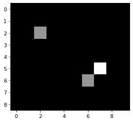
For demonstrating the principle of convolution, we first define an example image that’s rather simple.

image = np.asarray([
  [0, 0, 0, 0, 0, 0, 0, 0, 0, 0],
  [0, 0, 0, 0, 0, 0, 0, 0, 0, 0],
  [0, 0, 1, 0, 0, 0, 0, 0, 0, 0],
  [0, 0, 0, 0, 0, 0, 0, 0, 0, 0],
  [0, 0, 0, 0, 0, 0, 0, 0, 0, 0],
  [0, 0, 0, 0, 0, 0, 0, 2, 0, 0],
  [0, 0, 0, 0, 0, 0, 1, 0, 0, 0],
  [0, 0, 0, 0, 0, 0, 0, 0, 0, 0],
  [0, 0, 0, 0, 0, 0, 0, 0, 0, 0]
]).astype(float)

imshow(image)

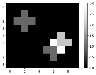
Next, we define a simple convolution kernel, that is represented by a small image.

kernel = np.asarray([
  [0, 1, 0],
  [1, 1, 1],
  [0, 1, 0],
])

Next, we convolve the image with the kernel using scipy.ndimage.convolve. When we print out the result, we can see how a 1 in the original image spreads, because for every directly neighboring pixel, the kernel sums the neighbor intensities. If there are multuple pixels with intensity > 0 in the original image, the resulting image will in their neighborhood compute the sum. You could call this kernel a local sum-kernel.

convolved = convolve(image, kernel)

imshow(convolved, colorbar=True)

convolved

array([[0., 0., 0., 0., 0., 0., 0., 0., 0., 0.],
       [0., 0., 1., 0., 0., 0., 0., 0., 0., 0.],
       [0., 1., 1., 1., 0., 0., 0., 0., 0., 0.],
       [0., 0., 1., 0., 0., 0., 0., 0., 0., 0.],
       [0., 0., 0., 0., 0., 0., 0., 2., 0., 0.],
       [0., 0., 0., 0., 0., 0., 3., 2., 2., 0.],
       [0., 0., 0., 0., 0., 1., 1., 3., 0., 0.],
       [0., 0., 0., 0., 0., 0., 1., 0., 0., 0.],
       [0., 0., 0., 0., 0., 0., 0., 0., 0., 0.]])

Other kernels

Depending on which kerne is used for the convolution, the images can look quite differently. A mean-kernel for example computes the average pixel intensity locally:

mean_kernel = np.asarray([
  [0, 0.2, 0],
  [0.2, 0.2, 0.2],
  [0, 0.2, 0],
])

mean_convolved = convolve(image, mean_kernel)

imshow(mean_convolved, colorbar=True)

mean_convolved

array([[0. , 0. , 0. , 0. , 0. , 0. , 0. , 0. , 0. , 0. ],
       [0. , 0. , 0.2, 0. , 0. , 0. , 0. , 0. , 0. , 0. ],
       [0. , 0.2, 0.2, 0.2, 0. , 0. , 0. , 0. , 0. , 0. ],
       [0. , 0. , 0.2, 0. , 0. , 0. , 0. , 0. , 0. , 0. ],
       [0. , 0. , 0. , 0. , 0. , 0. , 0. , 0.4, 0. , 0. ],
       [0. , 0. , 0. , 0. , 0. , 0. , 0.6, 0.4, 0.4, 0. ],
       [0. , 0. , 0. , 0. , 0. , 0.2, 0.2, 0.6, 0. , 0. ],
       [0. , 0. , 0. , 0. , 0. , 0. , 0.2, 0. , 0. , 0. ],
       [0. , 0. , 0. , 0. , 0. , 0. , 0. , 0. , 0. , 0. ]])

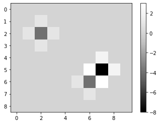
The following kernel is a simple form of a Laplace operator.

laplace_operator = np.asarray([
  [0, 1, 0],
  [1, -4, 1],
  [0, 1, 0],
])

laplacian = convolve(image, laplace_operator)

imshow(laplacian, colorbar=True)

laplacian

array([[ 0.,  0.,  0.,  0.,  0.,  0.,  0.,  0.,  0.,  0.],
       [ 0.,  0.,  1.,  0.,  0.,  0.,  0.,  0.,  0.,  0.],
       [ 0.,  1., -4.,  1.,  0.,  0.,  0.,  0.,  0.,  0.],
       [ 0.,  0.,  1.,  0.,  0.,  0.,  0.,  0.,  0.,  0.],
       [ 0.,  0.,  0.,  0.,  0.,  0.,  0.,  2.,  0.,  0.],
       [ 0.,  0.,  0.,  0.,  0.,  0.,  3., -8.,  2.,  0.],
       [ 0.,  0.,  0.,  0.,  0.,  1., -4.,  3.,  0.,  0.],
       [ 0.,  0.,  0.,  0.,  0.,  0.,  1.,  0.,  0.,  0.],
       [ 0.,  0.,  0.,  0.,  0.,  0.,  0.,  0.,  0.,  0.]])

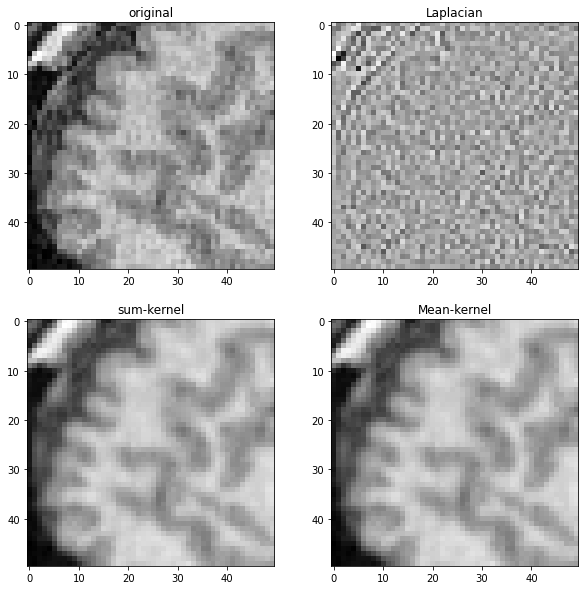
To demonstrate what these different kernels do, we apply them to the MRI image shown before.

# open dataset and extract single plane
noisy_mri = imread('../../data/Haase_MRT_tfl3d1.tif')[90].astype(float)

# zoom in by cropping a part out
noisy_mri_zoom = noisy_mri[50:100, 50:100]

convolved_mri = convolve(noisy_mri_zoom, kernel)
mean_mri = convolve(noisy_mri_zoom, mean_kernel)
laplacian_mri = convolve(noisy_mri_zoom, laplace_operator)

fig, axes = plt.subplots(2, 2, figsize=(10,10))

imshow(noisy_mri_zoom, plot=axes[0,0])
axes[0,0].set_title("original")
imshow(laplacian_mri, plot=axes[0,1])
axes[0,1].set_title("Laplacian")
imshow(convolved_mri, plot=axes[1,0])
axes[1,0].set_title("sum-kernel")
imshow(mean_mri, plot=axes[1,1])
axes[1,1].set_title("Mean-kernel")

Text(0.5, 1.0, 'Mean-kernel')