Quantitative image analysis#
After segmenting and labeling objects in an image, we can measure properties of these objects.
See also
Before we can do measurements, we need an image and a corresponding label_image. Therefore, we recapitulate filtering, thresholding and labeling:
from skimage.io import imread
from skimage import filters
from skimage import measure
from pyclesperanto_prototype import imshow
import pandas as pd
import numpy as np
# load image
image = imread("../../data/blobs.tif")
# denoising
blurred_image = filters.gaussian(image, sigma=1)
# binarization
threshold = filters.threshold_otsu(blurred_image)
thresholded_image = blurred_image >= threshold
# labeling
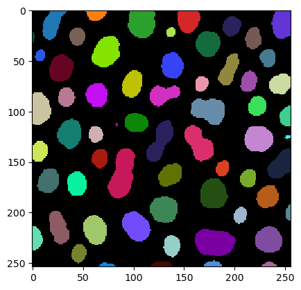
label_image = measure.label(thresholded_image)
# visualization
imshow(label_image, labels=True)
Measurements / region properties#
To read out properties from regions, we use the regionprops function:
# analyse objects
properties = measure.regionprops(label_image, intensity_image=image)
The results are stored as RegionProps objects, which are not very informative:
properties[0:5]
[<skimage.measure._regionprops.RegionProperties at 0x1c272b8f8e0>,
 <skimage.measure._regionprops.RegionProperties at 0x1c26d278af0>,
 <skimage.measure._regionprops.RegionProperties at 0x1c26d2784c0>,
 <skimage.measure._regionprops.RegionProperties at 0x1c26d278b20>,
 <skimage.measure._regionprops.RegionProperties at 0x1c26d278b80>]
If you are interested which properties we measured: They are listed in the documentation of the measure.regionprops function. Basically, we now have a variable properties which contains 40 different features. But we are only interested in a small subset of them.
Therefore, we can reorganize the measurements into a dictionary containing arrays with our features of interest:
statistics = {
    'area':       [p.area               for p in properties],
    'mean':       [p.mean_intensity     for p in properties],
    'major_axis': [p.major_axis_length  for p in properties],
    'minor_axis': [p.minor_axis_length for p in properties]
}
Reading those dictionaries of arrays is not very convenient. For that we introduce pandas DataFrames which are commonly used by data scientists. “DataFrames” is just another term for “tables” used in Python.
df = pd.DataFrame(statistics)
df
| area | mean | major_axis | minor_axis | |
|---|---|---|---|---|
| 0 | 429 | 191.440559 | 34.779230 | 16.654732 |
| 1 | 183 | 179.846995 | 20.950530 | 11.755645 |
| 2 | 658 | 205.604863 | 30.198484 | 28.282790 |
| 3 | 433 | 217.515012 | 24.508791 | 23.079220 |
| 4 | 472 | 213.033898 | 31.084766 | 19.681190 |
| ... | ... | ... | ... | ... |
| 57 | 213 | 184.525822 | 18.753879 | 14.468993 |
| 58 | 79 | 184.810127 | 18.287489 | 5.762488 |
| 59 | 88 | 182.727273 | 21.673692 | 5.389867 |
| 60 | 52 | 189.538462 | 14.335104 | 5.047883 |
| 61 | 48 | 173.833333 | 16.925660 | 3.831678 |
62 rows × 4 columns
You can also add custom columns by computing your own metric, for example the aspect_ratio:
df['aspect_ratio'] = [p.major_axis_length / p.minor_axis_length for p in properties]
df
| area | mean | major_axis | minor_axis | aspect_ratio | |
|---|---|---|---|---|---|
| 0 | 429 | 191.440559 | 34.779230 | 16.654732 | 2.088249 |
| 1 | 183 | 179.846995 | 20.950530 | 11.755645 | 1.782168 |
| 2 | 658 | 205.604863 | 30.198484 | 28.282790 | 1.067734 |
| 3 | 433 | 217.515012 | 24.508791 | 23.079220 | 1.061942 |
| 4 | 472 | 213.033898 | 31.084766 | 19.681190 | 1.579415 |
| ... | ... | ... | ... | ... | ... |
| 57 | 213 | 184.525822 | 18.753879 | 14.468993 | 1.296143 |
| 58 | 79 | 184.810127 | 18.287489 | 5.762488 | 3.173540 |
| 59 | 88 | 182.727273 | 21.673692 | 5.389867 | 4.021193 |
| 60 | 52 | 189.538462 | 14.335104 | 5.047883 | 2.839825 |
| 61 | 48 | 173.833333 | 16.925660 | 3.831678 | 4.417297 |
62 rows × 5 columns
Those dataframes can be saved to disk conveniently:
df.to_csv("blobs_analysis.csv")
Furthermore, one can measure properties from our statistics table using numpy. For example the mean area:
# measure mean area
np.mean(df['area'])
355.3709677419355
Exercises#
Analyse the loaded blobs image.
How many objects are in it?
How large is the largest object?
What are mean and standard deviation of the image?
What are mean and standard deviation of the area of the segmented objects?