Computing with images

We have seen in the last chapter that images exist in the form of Numpy arrays. We will here see different types of image processing computations that we can do with such arrays such as arithmetic operations, combining images etc.

We have seen in the last chapter that we could create images using e.g. the np.random.random function. Let’s create two tiny images:

import numpy as np
from matplotlib import pyplot as plt

image1 = np.ones((3,5))
image1

array([[1., 1., 1., 1., 1.],
       [1., 1., 1., 1., 1.],
       [1., 1., 1., 1., 1.]])

image2 = np.random.random((3,5))
image2

array([[0.1389824 , 0.99979463, 0.82577042, 0.79474507, 0.23101268],
       [0.27034647, 0.01410389, 0.20435784, 0.0721552 , 0.61984191],
       [0.85459468, 0.58800162, 0.62462822, 0.01819988, 0.06607906]])

Simple calculus

As a recap from last chapter, we have seen that we can do arithemtics with images just as we would with simple numbers:

image1_plus = image1 + 3
image1_plus

array([[4., 4., 4., 4., 4.],
       [4., 4., 4., 4., 4.],
       [4., 4., 4., 4., 4.]])

This is valid for all basis operations like addition, multiplication etc. Even raising to a given power works:

image1_plus ** 2

array([[16., 16., 16., 16., 16.],
       [16., 16., 16., 16., 16.],
       [16., 16., 16., 16., 16.]])

Combining images

If images have the same size, we can here again treat them like simple numbers and do maths with them: again addition, multiplication etc. For example:

image1 + image2

array([[1.1389824 , 1.99979463, 1.82577042, 1.79474507, 1.23101268],
       [1.27034647, 1.01410389, 1.20435784, 1.0721552 , 1.61984191],
       [1.85459468, 1.58800162, 1.62462822, 1.01819988, 1.06607906]])

Functions pixel by pixel

In addition of allowing us to create various types of arrays, Numpy also provides us functions that can operate on arrays. In many cases, the input is an image and the output is an image of the same size where a given function has been applied to each individual pixel.

For example we might want to apply a log function to an image to reduce the range of values that pixels can take. Here we would use the np.log function:

np.log(image2)

array([[-1.97340794e+00, -2.05388747e-04, -1.91438488e-01,
        -2.29733884e-01, -1.46528267e+00],
       [-1.30805091e+00, -4.26130469e+00, -1.58788269e+00,
        -2.62893591e+00, -4.78290819e-01],
       [-1.57127986e-01, -5.31025584e-01, -4.70598659e-01,
        -4.00634024e+00, -2.71690330e+00]])

As we can see the input image had 3 rows and 5 columns and the output image has the same dimensions. You can find many functions in Numpy that operate this way e.g. to take an exponential (np.exp()), to do trigonometry (np.cos(), np.sin()) etc.

Image statistics

Another type of functions takes an image as input but returns an output of a different size by computing a statistic on the image or parts of it. For example we can compute the average of all image2 pixel values:

np.mean(image2)

0.4215075982440046

Or we can specify that we want to compute the mean along a certain dimension of the image, in 2D along columns or rows. Let’s keep in mind what image2 is:

image2

array([[0.1389824 , 0.99979463, 0.82577042, 0.79474507, 0.23101268],
       [0.27034647, 0.01410389, 0.20435784, 0.0721552 , 0.61984191],
       [0.85459468, 0.58800162, 0.62462822, 0.01819988, 0.06607906]])

Now we take the average over columns, which means along the first axis or axis=0:

np.mean(image2, axis=0)

array([0.42130785, 0.53396671, 0.55158549, 0.29503338, 0.30564455])

The same logic applies to all other statistical functions such as taking the minium (np.min()), the maxiumum (np.max()), standard deviation (np.std()), median (np.median()) etc.

Note that most of this function can also be called directly on the Numpy array variable. For example

np.std(image2)

0.3362691013424119

and

image2.std()

0.3362691013424119

are completely equivalent. In the latter case using the dot notation, you might hear that std() is a method of image2.

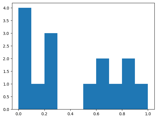
Finally we might want to have a look at the actual distribution of pixel values. For this we take a look at the histogram of the image.

number_of_bins = 10
min_max = [0,1]
histogram,bins = np.histogram(image2.ravel(),number_of_bins,min_max)

plt.hist(image2.ravel(), number_of_bins, min_max)
plt.show()

Exercise

From the numpy.random module, find a function that generates Poisson noise and creata a 4x9 image. Compute its mean and standard deviation.