Object classification with scikit-learn#
Based on size and shape measurements, e.g. derived using scikit-image regionprops and some sparse ground truth annotation, we can classify objects. A common algorithm for this are Random Forest Classifiers. A commonly used implementation is available as scikit-learn Random Forest Classifier.
See also
from sklearn.ensemble import RandomForestClassifier

from skimage.io import imread
from pyclesperanto_prototype import imshow, replace_intensities, relabel_sequential
from skimage.filters import threshold_otsu
from skimage.measure import label, regionprops
from skimage.segmentation import clear_border
import numpy as np
import pandas as pd
import matplotlib.pyplot as plt
Our starting point are an image, a label image and some ground truth annotation. The annotation is also a label image where the user was just drawing lines with different intensity (class) through small objects, large objects and elongated objects.
# load and label data
image = imread('../../data/blobs.tif')
labels = label(image > threshold_otsu(image))
annotation = imread('../../data/label_annotation.tif')

# visualize
fig, ax = plt.subplots(1,3, figsize=(15,15))
imshow(image, plot=ax[0])
imshow(labels, plot=ax[1], labels=True)
imshow(image, plot=ax[2], continue_drawing=True)
imshow(annotation, plot=ax[2], alpha=0.7, labels=True)
Feature extraction#
The first step to classify objects according to their properties is feature extraction.
stats = regionprops(labels, intensity_image=image)

# read out specific measurements
label_ids =          np.asarray([s.label for s in stats])
areas =              np.asarray([s.area for s in stats])
minor_axis_lengths = np.asarray([s.minor_axis_length for s in stats])
major_axis_lengths = np.asarray([s.major_axis_length for s in stats])

# compute additional parameters
aspect_ratios = major_axis_lengths / minor_axis_lengths
/var/folders/p1/6svzckgd1y5906pfgm71fvmr0000gn/T/ipykernel_18924/1513904267.py:10: RuntimeWarning: invalid value encountered in true_divide
  aspect_ratios = major_axis_lengths / minor_axis_lengths
We also read out the maximum intensity of every labeled object from the ground truth annotation. These values will serve to train the classifier.
annotation_stats = regionprops(labels, intensity_image=annotation)

annotated_class = np.asarray([s.max_intensity for s in annotation_stats])
Data wrangling#
To look at the data before it is fed to the training, we visualize it as pandas DataFrame. Note: The rows with annotated_class=0 correspond to labels that have not been annotated.
data = {
    'label': label_ids,
    'area': areas,
    'minor_axis': minor_axis_lengths,
    'major_axis': major_axis_lengths,
    'aspect_ratio': aspect_ratios,
    'annotated_class': annotated_class
}

table = pd.DataFrame(data)

# show only first 5 rows
table.iloc[:5]
| label | area | minor_axis | major_axis | aspect_ratio | annotated_class | |
|---|---|---|---|---|---|---|
| 0 | 1 | 433 | 16.819060 | 34.957399 | 2.078439 | 0.0 |
| 1 | 2 | 185 | 11.803854 | 21.061417 | 1.784283 | 0.0 |
| 2 | 3 | 658 | 28.278264 | 30.212552 | 1.068402 | 2.0 |
| 3 | 4 | 434 | 23.064079 | 24.535398 | 1.063793 | 0.0 |
| 4 | 5 | 477 | 19.833058 | 31.162612 | 1.571246 | 0.0 |
From that table, we extract now a table that only contains the annotated rows/labels.
annotated_table = table[table['annotated_class'] > 0]
annotated_table
| label | area | minor_axis | major_axis | aspect_ratio | annotated_class | |
|---|---|---|---|---|---|---|
| 2 | 3 | 658 | 28.278264 | 30.212552 | 1.068402 | 2.0 |
| 6 | 7 | 81 | 9.239435 | 11.153514 | 1.207164 | 2.0 |
| 10 | 11 | 501 | 24.403675 | 26.232105 | 1.074924 | 3.0 |
| 14 | 15 | 448 | 21.751312 | 26.272749 | 1.207870 | 3.0 |
| 17 | 18 | 425 | 19.335056 | 28.075209 | 1.452037 | 3.0 |
| 21 | 22 | 412 | 21.819832 | 24.135300 | 1.106118 | 3.0 |
| 26 | 27 | 676 | 24.623036 | 36.525858 | 1.483402 | 1.0 |
| 30 | 31 | 610 | 17.433716 | 48.005150 | 2.753581 | 1.0 |
| 31 | 32 | 14 | 4.120630 | 4.208834 | 1.021406 | 2.0 |
| 32 | 33 | 641 | 21.042345 | 40.781012 | 1.938045 | 1.0 |
| 35 | 36 | 22 | 4.355578 | 6.495072 | 1.491208 | 2.0 |
| 37 | 38 | 902 | 21.741393 | 54.785426 | 2.519867 | 1.0 |
As we do not want to use all columns for training, we now select the right columns. It is recommended to write a short convenience function select_data for this, because we will reuse it later for prediction.
def select_data(table):
    return np.asarray([
        table['area'],
        table['aspect_ratio']
    ])

training_data = select_data(annotated_table).T
training_data
array([[658.        ,   1.06840194],
       [ 81.        ,   1.20716407],
       [501.        ,   1.07492436],
       [448.        ,   1.20786966],
       [425.        ,   1.45203663],
       [412.        ,   1.1061176 ],
       [676.        ,   1.48340188],
       [610.        ,   2.75358106],
       [ 14.        ,   1.02140552],
       [641.        ,   1.93804502],
       [ 22.        ,   1.4912077 ],
       [902.        ,   2.51986728]])
We also extract the annotation from that table and call it ground_truth.
ground_truth = annotated_table['annotated_class'].tolist()
ground_truth
[2.0, 2.0, 3.0, 3.0, 3.0, 3.0, 1.0, 1.0, 2.0, 1.0, 2.0, 1.0]
Classifier Training#
Next, we can train the Random Forest Classifer. It needs training data and ground truth in the format presented above.
classifier = RandomForestClassifier(max_depth=2, n_estimators=10, random_state=0)
classifier.fit(training_data, ground_truth)
RandomForestClassifier(max_depth=2, n_estimators=10, random_state=0)
Prediction#
To apply a classifier to the whole dataset, or any other dataset, we need to bring the data into the same format as used for training. We can reuse the function select_data for that. Furthermore, we need to drop rows from our table where not-a-number (NaN) values appeared (read more).
table_without_nans = table.dropna(how="any")

all_data = select_data(table_without_nans).T
all_data
array([[433.        ,   2.0784395 ],
       [185.        ,   1.78428301],
       [658.        ,   1.06840194],
       [434.        ,   1.06379267],
       [477.        ,   1.57124594],
       [285.        ,   1.15397362],
       [ 81.        ,   1.20716407],
       [278.        ,   1.39040997],
       [231.        ,   1.14134293],
       [ 30.        ,   4.64290752],
       [501.        ,   1.07492436],
       [660.        ,   1.33770096],
       [ 99.        ,   1.27265076],
       [228.        ,   1.1427708 ],
       [448.        ,   1.20786966],
       [401.        ,   2.50541908],
       [520.        ,   1.18241662],
       [425.        ,   1.45203663],
       [271.        ,   1.34918562],
       [350.        ,   1.16890653],
       [159.        ,   1.22661614],
       [412.        ,   1.1061176 ],
       [426.        ,   1.81249164],
       [260.        ,   1.15413724],
       [506.        ,   1.6790716 ],
       [289.        ,   1.13174859],
       [676.        ,   1.48340188],
       [175.        ,   1.7693589 ],
       [361.        ,   1.22276182],
       [545.        ,   1.22505758],
       [610.        ,   2.75358106],
       [ 14.        ,   1.02140552],
       [641.        ,   1.93804502],
       [195.        ,   1.14814639],
       [593.        ,   1.08971368],
       [ 22.        ,   1.4912077 ],
       [268.        ,   1.29513144],
       [902.        ,   2.51986728],
       [473.        ,   1.74526337],
       [239.        ,   1.21436236],
       [167.        ,   1.29262079],
       [413.        ,   1.37572589],
       [415.        ,   1.2468234 ],
       [244.        ,   1.13831252],
       [377.        ,   1.28619722],
       [652.        ,   1.11512228],
       [379.        ,   1.14903134],
       [578.        ,   1.05037771],
       [ 69.        ,   3.02058993],
       [170.        ,   1.36058208],
       [472.        ,   2.04509462],
       [613.        ,   1.35438231],
       [543.        ,   1.3209039 ],
       [204.        ,   2.23080499],
       [555.        ,   1.07333913],
       [858.        ,   1.56519017],
       [281.        ,   1.32328162],
       [215.        ,   1.30875672],
       [  3.        ,   1.73205081],
       [ 81.        ,   3.13450027],
       [ 90.        ,   4.18288936],
       [ 53.        ,   2.92386162],
       [ 49.        ,   4.45617521]])
We can then hand over all_data to the classifier for prediction.
table_without_nans['predicted_class'] = classifier.predict(all_data)
print(table_without_nans['predicted_class'].tolist())
[1.0, 1.0, 2.0, 3.0, 3.0, 3.0, 2.0, 3.0, 2.0, 1.0, 3.0, 3.0, 2.0, 2.0, 3.0, 1.0, 3.0, 3.0, 3.0, 3.0, 2.0, 3.0, 1.0, 3.0, 3.0, 3.0, 3.0, 1.0, 3.0, 3.0, 1.0, 2.0, 1.0, 2.0, 2.0, 3.0, 3.0, 1.0, 1.0, 2.0, 2.0, 3.0, 3.0, 2.0, 3.0, 2.0, 3.0, 2.0, 1.0, 3.0, 1.0, 3.0, 3.0, 1.0, 3.0, 3.0, 3.0, 2.0, 1.0, 1.0, 1.0, 1.0, 1.0]
/var/folders/p1/6svzckgd1y5906pfgm71fvmr0000gn/T/ipykernel_18924/549567337.py:1: SettingWithCopyWarning:
A value is trying to be set on a copy of a slice from a DataFrame.
Try using .loc[row_indexer,col_indexer] = value instead

See the caveats in the documentation: https://pandas.pydata.org/pandas-docs/stable/user_guide/indexing.html#returning-a-view-versus-a-copy
  table_without_nans['predicted_class'] = classifier.predict(all_data)
We can then merge the table containing the predicted_class column with the original table. In the resulting table_with_prediction, we still need to decide how to handle NaN values. It is not possible to classify those because measurements are missing. Thus, we replace the class of those with 0 using fillna.
# merge prediction with original table
table_with_prediction = table.merge(table_without_nans, how='outer', on='label')
# replace not predicted (NaN) with 0
table_with_prediction['predicted_class'] = table_with_prediction['predicted_class'].fillna(0)

table_with_prediction
| label | area_x | minor_axis_x | major_axis_x | aspect_ratio_x | annotated_class_x | area_y | minor_axis_y | major_axis_y | aspect_ratio_y | annotated_class_y | predicted_class | |
|---|---|---|---|---|---|---|---|---|---|---|---|---|
| 0 | 1 | 433 | 16.819060 | 34.957399 | 2.078439 | 0.0 | 433.0 | 16.819060 | 34.957399 | 2.078439 | 0.0 | 1.0 |
| 1 | 2 | 185 | 11.803854 | 21.061417 | 1.784283 | 0.0 | 185.0 | 11.803854 | 21.061417 | 1.784283 | 0.0 | 1.0 |
| 2 | 3 | 658 | 28.278264 | 30.212552 | 1.068402 | 2.0 | 658.0 | 28.278264 | 30.212552 | 1.068402 | 2.0 | 2.0 |
| 3 | 4 | 434 | 23.064079 | 24.535398 | 1.063793 | 0.0 | 434.0 | 23.064079 | 24.535398 | 1.063793 | 0.0 | 3.0 |
| 4 | 5 | 477 | 19.833058 | 31.162612 | 1.571246 | 0.0 | 477.0 | 19.833058 | 31.162612 | 1.571246 | 0.0 | 3.0 |
| ... | ... | ... | ... | ... | ... | ... | ... | ... | ... | ... | ... | ... |
| 59 | 60 | 1 | 0.000000 | 0.000000 | NaN | 0.0 | NaN | NaN | NaN | NaN | NaN | 0.0 |
| 60 | 61 | 81 | 5.920690 | 18.558405 | 3.134500 | 0.0 | 81.0 | 5.920690 | 18.558405 | 3.134500 | 0.0 | 1.0 |
| 61 | 62 | 90 | 5.369081 | 22.458271 | 4.182889 | 0.0 | 90.0 | 5.369081 | 22.458271 | 4.182889 | 0.0 | 1.0 |
| 62 | 63 | 53 | 5.065719 | 14.811463 | 2.923862 | 0.0 | 53.0 | 5.065719 | 14.811463 | 2.923862 | 0.0 | 1.0 |
| 63 | 64 | 49 | 3.843548 | 17.127524 | 4.456175 | 0.0 | 49.0 | 3.843548 | 17.127524 | 4.456175 | 0.0 | 1.0 |
64 rows × 12 columns
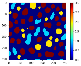
From that table, we can extract the column containing the prediction and use replace_intensities to generate a class_image. The background and objects with NaNs in measurements will have value 0 in that image.
# we add a 0 for the class of background at the beginning
predicted_class = [0] + table_with_prediction['predicted_class'].tolist()
class_image = replace_intensities(labels, predicted_class)
imshow(class_image, colorbar=True, colormap='jet')