3D Image Segmentation

Image segmentation in 3D is challenging for several reasons: In many microscopy imaging techniques, image quality varies in space: For example intensity and/or contrast degrades the deeper you image inside a sample. Furthermore, touching nuclei are hard to differentiate in an automated way. Last but not least, anisotropy is difficult to handle depending on the applied algorithms and respective given parameters. Some algorithms, like the Voronoi-Otsu-Labeling approach demonstrated here, only work for isotropic data.

from skimage.io import imread
from pyclesperanto_prototype import imshow
import pyclesperanto_prototype as cle
import matplotlib.pyplot as plt

import napari
from napari.utils import nbscreenshot

# For 3D processing, powerful graphics
# processing units might be necessary
cle.select_device('TX')

<NVIDIA GeForce GTX 1650 with Max-Q Design on Platform: NVIDIA CUDA (1 refs)>

To demonstrate the workflow, we’re using cropped and resampled image data from the Broad Bio Image Challenge: Ljosa V, Sokolnicki KL, Carpenter AE (2012). Annotated high-throughput microscopy image sets for validation. Nature Methods 9(7):637 / doi. PMID: 22743765 PMCID: PMC3627348. Available at http://dx.doi.org/10.1038/nmeth.2083

input_image = imread("../../data/BMP4blastocystC3-cropped_resampled_8bit.tif")

voxel_size_x = 0.202
voxel_size_y = 0.202
voxel_size_z = 1

For visualisation purposes we show intensity projections along X, Y and Z.

def show(image_to_show, labels=False):
    """
    This function generates three projections: in X-, Y- and Z-direction and shows them.
    """
    projection_x = cle.maximum_x_projection(image_to_show)
    projection_y = cle.maximum_y_projection(image_to_show)
    projection_z = cle.maximum_z_projection(image_to_show)

    fig, axs = plt.subplots(1, 3, figsize=(15, 15))
    cle.imshow(projection_x, plot=axs[0], labels=labels)
    cle.imshow(projection_y, plot=axs[1], labels=labels)
    cle.imshow(projection_z, plot=axs[2], labels=labels)
    plt.show()

show(input_image)
print(input_image.shape)

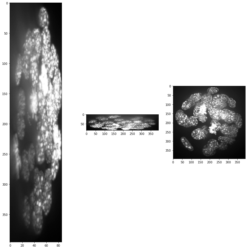
(86, 396, 393)

Obviously, voxel size is not isotropic. Thus, we scale the image with the voxel size used as scaling factor to get an image stack with isotropic voxels.

resampled = cle.scale(input_image, factor_x=voxel_size_x, factor_y=voxel_size_y, factor_z=voxel_size_z, auto_size=True)

show(resampled)
print(resampled.shape)

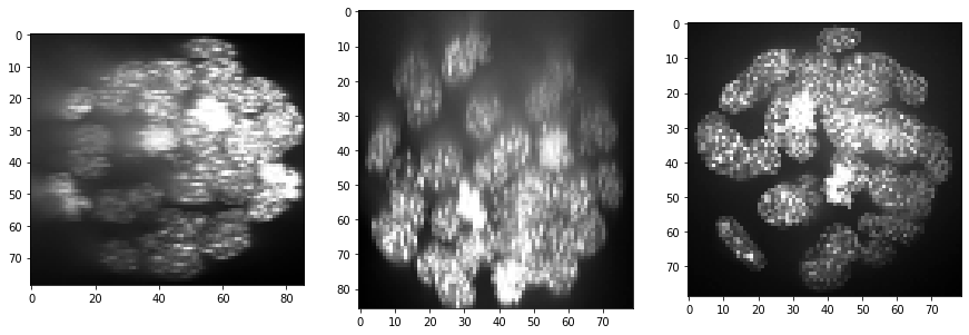
(86, 79, 79)

Intensity and background correction

As we can see, intensity is decreasing in Z-direction (from slice to slice) and contrast as well. At least the intensity decay can be corrected. In CLIJx, this method is known as equalize_mean_intensities_of_slices.

equalized_intensities_stack = cle.create_like(resampled)
a_slice = cle.create([resampled.shape[1], resampled.shape[0]])

num_slices = resampled.shape[0]
mean_intensity_stack = cle.mean_of_all_pixels(resampled)

corrected_slice = None
for z in range(0, num_slices):
    # get a single slice out of the stack
    cle.copy_slice(resampled, a_slice, z)
    # measure its intensity
    mean_intensity_slice = cle.mean_of_all_pixels(a_slice)
    # correct the intensity
    correction_factor = mean_intensity_slice/mean_intensity_stack
    corrected_slice = cle.multiply_image_and_scalar(a_slice, corrected_slice, correction_factor)
    # copy slice back in a stack
    cle.copy_slice(corrected_slice, equalized_intensities_stack, z)

show(equalized_intensities_stack)

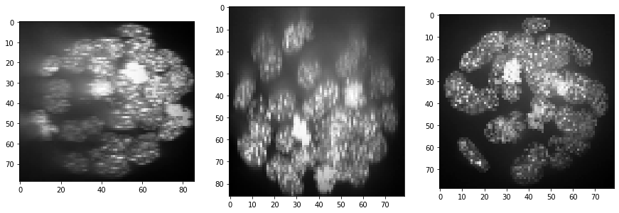
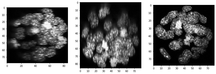
Furthermore, background intensity appears to increase, potentially a result if more scattering deep in the sample. We can compensate for that by using a background subtraction technique:

backgrund_subtracted = cle.top_hat_box(equalized_intensities_stack, radius_x=5, radius_y=5, radius_z=5)
show(backgrund_subtracted)

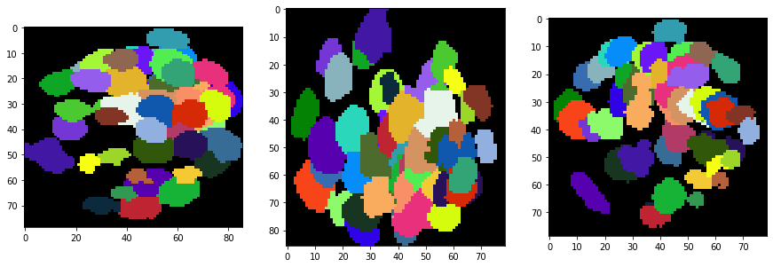
Segmentation

segmented = cle.voronoi_otsu_labeling(backgrund_subtracted, spot_sigma=3, outline_sigma=1)
show(segmented, labels=True)

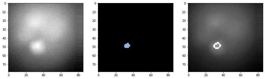
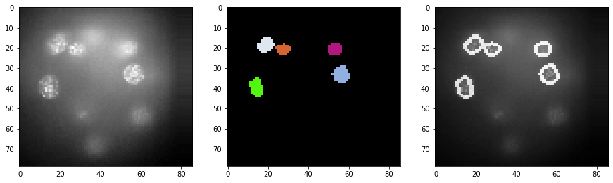
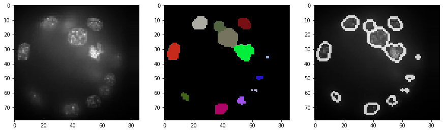
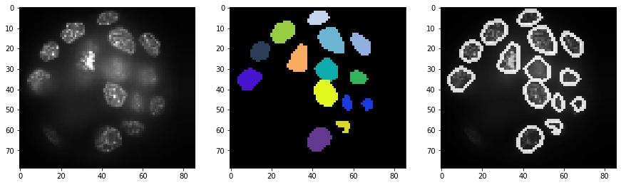
As segmentation results are hard to inspect in 3D, we generate an image stack with the original intensities + outlines of the segmentation. We show this stack for a couple of slices.

a_slice = cle.create([resampled.shape[1], resampled.shape[0]])
segmented_slice = cle.create([resampled.shape[1], resampled.shape[0]])

for z in range(0, resampled.shape[2], 20):
    label_outlines = None
    combined = None

    # get a single slice from the intensity image and the segmented label image
    cle.copy_slice(resampled, a_slice, z)
    cle.copy_slice(segmented, segmented_slice, z)

    # determine outlines around labeled objects
    label_outlines = cle.detect_label_edges(segmented_slice, label_outlines)

    # combine both images
    outline_intensity_factor = cle.maximum_of_all_pixels(a_slice)
    combined = cle.add_images_weighted(a_slice, label_outlines, combined, 1.0, outline_intensity_factor)

    # visualisation
    fig, axs = plt.subplots(1, 3, figsize=(15, 15))
    cle.imshow(a_slice, plot=axs[0])
    cle.imshow(segmented_slice, plot=axs[1], labels=True)
    cle.imshow(combined, plot=axs[2])

Visualization in 3D

For actual visualization in 3D you can also use napari.

# start napari
viewer = napari.Viewer()

# show images
viewer.add_image(cle.pull(resampled))
viewer.add_image(cle.pull(equalized_intensities_stack))
viewer.add_labels(cle.pull(segmented))

INFO:xmlschema:Resource 'XMLSchema.xsd' is already loaded

<Labels layer 'Labels' at 0x1eba6d51dc0>

viewer.dims.current_step = (40, 0, 0)
nbscreenshot(viewer)

INFO:OpenGL.acceleratesupport:No OpenGL_accelerate module loaded: No module named 'OpenGL_accelerate'

We can switch to a 3D view by clicking on the 3D button in the bottom left corner.

nbscreenshot(viewer)

We can then also tip and tilt the view.

nbscreenshot(viewer)