Statistics using Scikit-image#
We can use scikit-image for extracting features from label images. For convenience reasons we use the napari-skimage-regionprops library.
Before we can do measurements, we need an image and a corresponding label_image. Therefore, we recapitulate filtering, thresholding and labeling:
from skimage.io import imread
from skimage import filters
from skimage import measure
from napari_skimage_regionprops import regionprops_table
from pyclesperanto_prototype import imshow
import pandas as pd
import numpy as np
import pyclesperanto_prototype as cle
# load image
image = imread("../../data/blobs.tif")
# denoising
blurred_image = filters.gaussian(image, sigma=1)
# binarization
threshold = filters.threshold_otsu(blurred_image)
thresholded_image = blurred_image >= threshold
# labeling
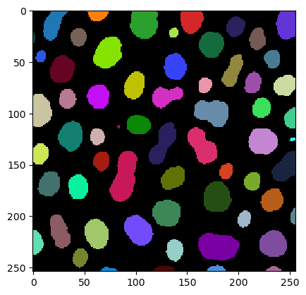
label_image = measure.label(thresholded_image)
# visualization
imshow(label_image, labels=True)
Measurements / region properties#
We are now using the very handy function regionprops_table. It provides features based on the scikit-image regionprops list of measurements library. Let us check first what we need to provide for this function:
regionprops_table?
Signature:
regionprops_table(
    image: 'napari.types.ImageData',
    labels: 'napari.types.LabelsData',
    size: bool = True,
    intensity: bool = True,
    perimeter: bool = False,
    shape: bool = False,
    position: bool = False,
    moments: bool = False,
    napari_viewer: 'napari.Viewer' = None,
) -> 'pandas.DataFrame'
Docstring: Adds a table widget to a given napari viewer with quantitative analysis results derived from an image-label pair.
File:      c:\users\maral\mambaforge\envs\feature_blogpost\lib\site-packages\napari_skimage_regionprops\_regionprops.py
Type:      function
We see that we need to provide which feature categories we want to measure. One way of dividing these categories is shown here:
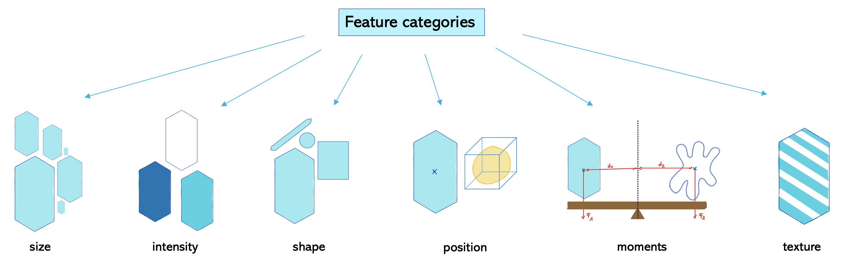
Feature categories which are set to True are measured by default. In this case, the categories are size and intensity. But perimeter and shape would be also interesting to investigate. So we need to set them to True as well.
df = pd.DataFrame(regionprops_table(image , label_image,
                                           perimeter = True,
                                           shape = True,
                                           position=True,
                                           moments=True))
df
| label | area | bbox_area | equivalent_diameter | convex_area | max_intensity | mean_intensity | min_intensity | perimeter | perimeter_crofton | ... | moments_hu-1 | moments_hu-2 | moments_hu-3 | moments_hu-4 | moments_hu-5 | moments_hu-6 | standard_deviation_intensity | aspect_ratio | roundness | circularity | |
|---|---|---|---|---|---|---|---|---|---|---|---|---|---|---|---|---|---|---|---|---|---|
| 0 | 1 | 429 | 750 | 23.371345 | 479 | 232.0 | 191.440559 | 128.0 | 89.012193 | 87.070368 | ... | 0.018445 | 0.000847 | 1.133411e-04 | 1.205336e-08 | -2.714451e-06 | 3.298765e-08 | 29.793138 | 2.088249 | 0.451572 | 0.680406 |
| 1 | 2 | 183 | 231 | 15.264430 | 190 | 224.0 | 179.846995 | 128.0 | 53.556349 | 53.456120 | ... | 0.010549 | 0.001177 | 6.734903e-05 | -1.483503e-08 | -5.401836e-06 | -1.180484e-08 | 21.270534 | 1.782168 | 0.530849 | 0.801750 |
| 2 | 3 | 658 | 756 | 28.944630 | 673 | 248.0 | 205.604863 | 120.0 | 95.698485 | 93.409370 | ... | 0.000113 | 0.000104 | 1.146642e-06 | 4.801450e-13 | 9.889775e-09 | -1.248247e-11 | 29.392255 | 1.067734 | 0.918683 | 0.902871 |
| 3 | 4 | 433 | 529 | 23.480049 | 445 | 248.0 | 217.515012 | 120.0 | 77.455844 | 76.114262 | ... | 0.000096 | 0.000348 | 3.349309e-07 | -3.612652e-12 | 2.526209e-09 | -9.198337e-14 | 35.852345 | 1.061942 | 0.917813 | 0.906963 |
| 4 | 5 | 472 | 551 | 24.514670 | 486 | 248.0 | 213.033898 | 128.0 | 83.798990 | 82.127941 | ... | 0.005876 | 0.000072 | 4.356690e-06 | -6.223212e-11 | -3.178823e-07 | 4.522442e-11 | 28.741080 | 1.579415 | 0.621952 | 0.844645 |
| ... | ... | ... | ... | ... | ... | ... | ... | ... | ... | ... | ... | ... | ... | ... | ... | ... | ... | ... | ... | ... | ... |
| 57 | 58 | 213 | 285 | 16.468152 | 221 | 224.0 | 184.525822 | 120.0 | 52.284271 | 52.250114 | ... | 0.001745 | 0.000002 | 1.126452e-07 | 5.814575e-14 | 4.625041e-09 | -6.410600e-15 | 28.255467 | 1.296143 | 0.771094 | 0.979146 |
| 58 | 59 | 79 | 108 | 10.029253 | 84 | 248.0 | 184.810127 | 128.0 | 39.313708 | 39.953250 | ... | 0.056792 | 0.001777 | 1.725200e-04 | -5.364882e-08 | -2.906455e-05 | -7.903632e-08 | 33.739912 | 3.173540 | 0.300766 | 0.642316 |
| 59 | 60 | 88 | 110 | 10.585135 | 92 | 216.0 | 182.727273 | 128.0 | 45.692388 | 46.196967 | ... | 0.097966 | 0.002268 | 2.994111e-04 | -1.724577e-08 | -3.731912e-05 | -2.461160e-07 | 24.417173 | 4.021193 | 0.238521 | 0.529669 |
| 60 | 61 | 52 | 75 | 8.136858 | 56 | 248.0 | 189.538462 | 128.0 | 30.692388 | 32.924135 | ... | 0.046813 | 0.003694 | 3.041106e-04 | -2.539652e-07 | -5.698262e-05 | -1.984555e-07 | 37.867411 | 2.839825 | 0.322190 | 0.693668 |
| 61 | 62 | 48 | 68 | 7.817640 | 53 | 224.0 | 173.833333 | 128.0 | 33.071068 | 35.375614 | ... | 0.125246 | 0.004295 | 1.300612e-03 | 2.775191e-06 | 3.027878e-04 | 1.321910e-06 | 27.987596 | 4.417297 | 0.213334 | 0.551512 |
62 rows × 86 columns
As you can see, we have now plenty of features to investigate. We can print out all feature names with the keys function:
print(df.keys())
Index(['label', 'area', 'bbox_area', 'equivalent_diameter', 'convex_area',
       'max_intensity', 'mean_intensity', 'min_intensity', 'perimeter',
       'perimeter_crofton', 'extent', 'local_centroid-0', 'local_centroid-1',
       'solidity', 'feret_diameter_max', 'major_axis_length',
       'minor_axis_length', 'orientation', 'eccentricity', 'centroid-0',
       'centroid-1', 'bbox-0', 'bbox-1', 'bbox-2', 'bbox-3',
       'weighted_centroid-0', 'weighted_centroid-1', 'moments-0-0',
       'moments-0-1', 'moments-0-2', 'moments-0-3', 'moments-1-0',
       'moments-1-1', 'moments-1-2', 'moments-1-3', 'moments-2-0',
       'moments-2-1', 'moments-2-2', 'moments-2-3', 'moments-3-0',
       'moments-3-1', 'moments-3-2', 'moments-3-3', 'moments_normalized-0-0',
       'moments_normalized-0-1', 'moments_normalized-0-2',
       'moments_normalized-0-3', 'moments_normalized-1-0',
       'moments_normalized-1-1', 'moments_normalized-1-2',
       'moments_normalized-1-3', 'moments_normalized-2-0',
       'moments_normalized-2-1', 'moments_normalized-2-2',
       'moments_normalized-2-3', 'moments_normalized-3-0',
       'moments_normalized-3-1', 'moments_normalized-3-2',
       'moments_normalized-3-3', 'moments_central-0-0', 'moments_central-0-1',
       'moments_central-0-2', 'moments_central-0-3', 'moments_central-1-0',
       'moments_central-1-1', 'moments_central-1-2', 'moments_central-1-3',
       'moments_central-2-0', 'moments_central-2-1', 'moments_central-2-2',
       'moments_central-2-3', 'moments_central-3-0', 'moments_central-3-1',
       'moments_central-3-2', 'moments_central-3-3', 'moments_hu-0',
       'moments_hu-1', 'moments_hu-2', 'moments_hu-3', 'moments_hu-4',
       'moments_hu-5', 'moments_hu-6', 'standard_deviation_intensity',
       'aspect_ratio', 'roundness', 'circularity'],
      dtype='object')
And describe gives us basic statistics like max, mean, min and std of each feature:
df.describe()
| label | area | bbox_area | equivalent_diameter | convex_area | max_intensity | mean_intensity | min_intensity | perimeter | perimeter_crofton | ... | moments_hu-1 | moments_hu-2 | moments_hu-3 | moments_hu-4 | moments_hu-5 | moments_hu-6 | standard_deviation_intensity | aspect_ratio | roundness | circularity | |
|---|---|---|---|---|---|---|---|---|---|---|---|---|---|---|---|---|---|---|---|---|---|
| count | 62.000000 | 62.000000 | 62.000000 | 62.000000 | 62.000000 | 62.000000 | 62.000000 | 62.000000 | 62.000000 | 62.000000 | ... | 62.000000 | 6.200000e+01 | 6.200000e+01 | 6.200000e+01 | 6.200000e+01 | 6.200000e+01 | 62.000000 | 62.000000 | 62.000000 | 62.000000 |
| mean | 31.500000 | 355.370968 | 475.677419 | 20.074583 | 372.790323 | 233.548387 | 190.429888 | 125.161290 | 67.787235 | 67.071263 | ... | 0.012854 | 5.166382e-04 | 7.053581e-05 | 5.855846e-08 | 3.633047e-06 | -8.703715e-09 | 28.689171 | 1.637991 | 0.692418 | 0.894101 |
| std | 18.041619 | 211.367385 | 300.328169 | 7.091876 | 223.801078 | 19.371838 | 15.382559 | 4.602898 | 25.008581 | 23.507575 | ... | 0.027066 | 1.077748e-03 | 2.093454e-04 | 3.687535e-07 | 3.998053e-05 | 2.897240e-07 | 6.127700 | 0.794366 | 0.210973 | 0.183024 |
| min | 1.000000 | 7.000000 | 9.000000 | 2.985411 | 7.000000 | 152.000000 | 146.285714 | 112.000000 | 6.828427 | 9.155272 | ... | 0.000056 | 2.514436e-07 | 6.992073e-09 | -2.539652e-07 | -5.698262e-05 | -1.757113e-06 | 5.598834 | 1.048053 | 0.213334 | 0.529669 |
| 25% | 16.250000 | 194.750000 | 260.000000 | 15.745692 | 204.750000 | 232.000000 | 182.969505 | 120.000000 | 52.602291 | 52.551616 | ... | 0.000627 | 3.032838e-05 | 1.242304e-07 | -1.881559e-13 | -1.039790e-08 | -7.811552e-13 | 26.514258 | 1.168451 | 0.538616 | 0.805774 |
| 50% | 31.500000 | 366.000000 | 448.500000 | 21.585875 | 376.500000 | 240.000000 | 190.749492 | 128.000000 | 69.112698 | 68.204464 | ... | 0.001971 | 6.198102e-05 | 5.957846e-07 | 6.176303e-14 | 5.408146e-10 | -9.288753e-15 | 29.017801 | 1.316003 | 0.757485 | 0.925560 |
| 75% | 46.750000 | 500.750000 | 685.500000 | 25.250050 | 516.500000 | 248.000000 | 199.725305 | 128.000000 | 86.097980 | 84.307520 | ... | 0.010151 | 3.475818e-04 | 3.799021e-05 | 1.135209e-11 | 1.484276e-08 | 1.902152e-12 | 32.534123 | 1.769976 | 0.851463 | 0.966037 |
| max | 62.000000 | 896.000000 | 1350.000000 | 33.776066 | 977.000000 | 248.000000 | 220.026144 | 136.000000 | 129.982756 | 125.912897 | ... | 0.125246 | 5.440067e-03 | 1.300612e-03 | 2.775191e-06 | 3.027878e-04 | 1.321910e-06 | 38.323999 | 4.417297 | 0.974824 | 1.886542 |
8 rows × 86 columns
Exercises#
Make a table with only solidity, circularity and roundness.