Descriptive statistics of labeled images#
Using pandas and numpy, we can do basic descriptive statistics. Before we start, we derive some measurements from a labeled image.
import pandas as pd
import numpy as np
from skimage.io import imread, imshow
from napari_segment_blobs_and_things_with_membranes import gauss_otsu_labeling
from skimage.measure import regionprops_table
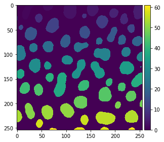
We load the image using scikit-image’s imread and segment it using Gauss-Otsu-Labeling.
image = imread('../../data/blobs.tif')
labels = gauss_otsu_labeling(image)
imshow(labels)
C:\Users\rober\miniconda3\envs\bio_39\lib\site-packages\skimage\io\_plugins\matplotlib_plugin.py:150: UserWarning: Low image data range; displaying image with stretched contrast.
  lo, hi, cmap = _get_display_range(image)
<matplotlib.image.AxesImage at 0x2819ae7b370>
From the labeled image we can derive descriptive intensity, size and shape statistics using scikit-image’s regionprops_table.
For post-processing the measurements, we turn them into a pandas Dataframe.
table = regionprops_table(labels, image, properties=['area', 'minor_axis_length', 'major_axis_length', 'eccentricity', 'feret_diameter_max'])
data_frame = pd.DataFrame(table)
data_frame
| area | minor_axis_length | major_axis_length | eccentricity | feret_diameter_max | |
|---|---|---|---|---|---|
| 0 | 422 | 16.488550 | 34.566789 | 0.878900 | 35.227830 |
| 1 | 182 | 11.736074 | 20.802697 | 0.825665 | 21.377558 |
| 2 | 661 | 28.409502 | 30.208433 | 0.339934 | 32.756679 |
| 3 | 437 | 23.143996 | 24.606130 | 0.339576 | 26.925824 |
| 4 | 476 | 19.852882 | 31.075106 | 0.769317 | 31.384710 |
| ... | ... | ... | ... | ... | ... |
| 56 | 211 | 14.522762 | 18.489138 | 0.618893 | 18.973666 |
| 57 | 78 | 6.028638 | 17.579799 | 0.939361 | 18.027756 |
| 58 | 86 | 5.426871 | 21.261427 | 0.966876 | 22.000000 |
| 59 | 51 | 5.032414 | 13.742079 | 0.930534 | 14.035669 |
| 60 | 46 | 3.803982 | 15.948714 | 0.971139 | 15.033296 |
61 rows × 5 columns
You can take a column out of the DataFrame. In this context it works like a Python dictionary.
data_frame["area"]
0     422
1     182
2     661
3     437
4     476
     ...
56    211
57     78
58     86
59     51
60     46
Name: area, Length: 61, dtype: int32
Even though this data structure appears more than just a vector, numpy is capable of applying basic descriptive statistics functions:
np.mean(data_frame["area"])
358.42622950819674
np.min(data_frame["area"])
5
np.max(data_frame["area"])
899
Individual cells of the DataFrame can be accessed like this:
data_frame["area"][0]
422
For loops can also iterate over table columns like this:
for area_value in data_frame["area"]:
    print(area_value)
422
182
661
437
476
277
259
219
67
19
486
630
221
78
449
516
390
419
267
353
151
400
426
246
503
278
681
176
358
544
597
181
629
596
5
263
899
476
233
164
394
411
235
375
654
376
579
64
161
457
625
535
205
562
845
280
211
78
86
51
46
Summary statistics with Pandas#
Pandas also allows you to visualize summary statistics of measurement using the describe() function.
data_frame.describe()
| area | minor_axis_length | major_axis_length | eccentricity | feret_diameter_max | |
|---|---|---|---|---|---|
| count | 61.000000 | 61.000000 | 61.000000 | 61.000000 | 61.000000 |
| mean | 358.426230 | 17.127032 | 24.796851 | 0.657902 | 25.323368 |
| std | 210.446942 | 6.587838 | 9.074265 | 0.189669 | 8.732456 |
| min | 5.000000 | 1.788854 | 3.098387 | 0.312788 | 3.162278 |
| 25% | 205.000000 | 14.319400 | 18.630719 | 0.503830 | 19.313208 |
| 50% | 375.000000 | 17.523565 | 23.768981 | 0.645844 | 24.698178 |
| 75% | 503.000000 | 21.753901 | 30.208433 | 0.825665 | 31.384710 |
| max | 899.000000 | 28.409502 | 54.500296 | 0.984887 | 52.201533 |
Correlation matrix#
If you want to learn which parameters are correlated with other parameters, you can visualize that using pandas’s corr().
data_frame.corr()
| area | minor_axis_length | major_axis_length | eccentricity | feret_diameter_max | |
|---|---|---|---|---|---|
| area | 1.000000 | 0.890649 | 0.895282 | -0.192147 | 0.916652 |
| minor_axis_length | 0.890649 | 1.000000 | 0.664507 | -0.566486 | 0.716706 |
| major_axis_length | 0.895282 | 0.664507 | 1.000000 | 0.168454 | 0.995196 |
| eccentricity | -0.192147 | -0.566486 | 0.168454 | 1.000000 | 0.103529 |
| feret_diameter_max | 0.916652 | 0.716706 | 0.995196 | 0.103529 | 1.000000 |
Exercise#
Process the banana dataset, e.g. using a for-loop that goes through the folder ../../data/banana/ and processes all the images. Segment all objects in the banana slice images and print out the largest area found for each slice. Collect these values in a list and visualize it as pandas DataFrame.