Images are arrays of numbers

Numpy is a library for processing multi-dimensional lists of numbers, of which microscopy images (stacks, multi-channel, time-lapses etc.) are a prominent example. We give here an introduction to this library.

See also

• Image manipulation and processing using Numpy and Scipy by Emmanuelle Gouillart and Gaël Varoquaux

import numpy as np
from matplotlib.pyplot import imshow

Numpy arrays

An image is just a two dimensional list of pixels values, in other words a matrix, with a certain number of rows and columns. Therefore we can define it as a list of lists, each list being a row of pixels:

raw_image_array = [
    [1, 0, 2, 1, 0, 0, 0],
    [0, 3, 1, 0, 1, 0, 1],
    [0, 5, 5, 1, 0, 1, 0],
    [0, 6, 6, 5, 1, 0, 2],
    [0, 0, 5, 6, 3, 0, 1],
    [0, 1, 2, 1, 0, 0, 1],
    [1, 0, 1, 0, 0, 1, 0]
]
raw_image_array

[[1, 0, 2, 1, 0, 0, 0],
 [0, 3, 1, 0, 1, 0, 1],
 [0, 5, 5, 1, 0, 1, 0],
 [0, 6, 6, 5, 1, 0, 2],
 [0, 0, 5, 6, 3, 0, 1],
 [0, 1, 2, 1, 0, 0, 1],
 [1, 0, 1, 0, 0, 1, 0]]

imshow(raw_image_array)

<matplotlib.image.AxesImage at 0x1f9fbdb4b80>

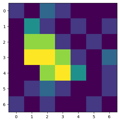
This output is almost the same as above with the difference that now it is indicated that we are dealing with a Numpy array. Such Numpy arrays can now be treated as a one entity and we can perform the computation that we coudn’t before:

image = np.asarray(raw_image_array)

image - 2

array([[-1, -2,  0, -1, -2, -2, -2],
       [-2,  1, -1, -2, -1, -2, -1],
       [-2,  3,  3, -1, -2, -1, -2],
       [-2,  4,  4,  3, -1, -2,  0],
       [-2, -2,  3,  4,  1, -2, -1],
       [-2, -1,  0, -1, -2, -2, -1],
       [-1, -2, -1, -2, -2, -1, -2]])

Note that these computations are very efficient because they are vectorized, i.e. they can in principle be performed in parallel.

Two important properties

Arrays like image have different properties. Two of the most important ones are:

• the shape of the array, i.e. the number of rows, columns (and channels, planes etc. for multi-dimensional images)

• the dtype of the array, i.e. an image of type int64 has 2 to the power of 64 different grey values.

image.shape

(7, 7)

image.dtype

dtype('int32')

Other ways of creating arrays

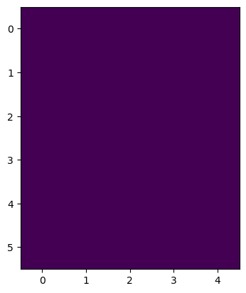
When working with images, we often create artifical images to see what filters do with them. For example, we can create an image where all pixels have value 0 but a single one using the Numpy function np.zeros. It requires to specify and image size.

image_size = (6, 5)

image1 = np.zeros(image_size)
image1

array([[0., 0., 0., 0., 0.],
       [0., 0., 0., 0., 0.],
       [0., 0., 0., 0., 0.],
       [0., 0., 0., 0., 0.],
       [0., 0., 0., 0., 0.],
       [0., 0., 0., 0., 0.]])

imshow(image1)

<matplotlib.image.AxesImage at 0x1f9fc000f10>

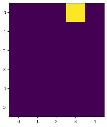
As images are just arrays, we just set pixel values as if we were accessing arrays. From this you also learn that the first axis (coordinate 0) is going from top to bottom while the second axis (coordinate 3) goes from left to right.

image1[0,3] = 1

imshow(image1)

<matplotlib.image.AxesImage at 0x1f9fbe7ad90>

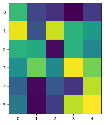
For studying noise, we can for example create an image with random values using np.random.random.

image_random = np.random.random((6, 5))
imshow(image_random)

<matplotlib.image.AxesImage at 0x1f9fbef72e0>