Clustering - a quick walkthrough

The term clustering stands for grouping objects according to their properties without providing any annotation. Algorithms in this field are also reffered to as unsupervised machine learning. The algorithms do receive input from the programmer though, e.g. by selecting specific measurements, which might render the term unsupervised in this context a bit misleading.

When clustering data retrieved from images, we use terms such as standard-scaling, dimensionality reduction and finally algorithms such as k-means clustering. This notebook is a quick walk through using these techniques before the methods are demonstrated in more detail in the following notebooks.

See also

• Explorative image data science with napari (FocalPlane blog post)

import pyclesperanto_prototype as cle
from napari_simpleitk_image_processing import label_statistics
from sklearn.preprocessing import StandardScaler
from sklearn.mixture import GaussianMixture
from sklearn.cluster import KMeans
import pandas as pd
import seaborn as sns
import seaborn
import numpy as np
import umap
import matplotlib.pyplot as plt
from skimage.data import human_mitosis

First we start by loading a 3D dataset showing a Tribolium castaneum embryo undergoing gastrulation (curtesy: Daniela Vorkel, Myers lab, MPI-CBG / CSBD Dresden). The dataset shows dense nuclei marked with nuclei-GFP on the left forming the embryo and less dense nuclei, called serosa, on the right surrounding the embryo.

image = cle.imread("../../data/Lund-25MB.tif")
image

cle._ image shape (116, 636, 354) dtype float32 size 99.6 MB min 0.0 max 255.0

We segment the nuclei as shown in earlier sections using top-hat-filtering for background removal and Voronoi-Otsu-Labeling.

background_subtracted = cle.top_hat_box(image, radius_x=5, radius_y=5)
nuclei_labels = cle.voronoi_otsu_labeling(background_subtracted, spot_sigma=1)
nuclei_labels

cle._ image shape (116, 636, 354) dtype uint32 size 99.6 MB min 0.0 max 1200.0

Feature extraction

We next measure properties such as intensity, size and shape from the labeled nuclei using napari-SimpleITK-image-processing.

statistics = label_statistics(image, nuclei_labels,
                             intensity=True,
                             perimeter=True,
                             shape=True)
statistics.keys()

Index(['label', 'maximum', 'mean', 'median', 'minimum', 'sigma', 'sum',
       'variance', 'elongation', 'feret_diameter', 'flatness', 'roundness',
       'equivalent_ellipsoid_diameter_0', 'equivalent_ellipsoid_diameter_1',
       'equivalent_ellipsoid_diameter_2', 'equivalent_spherical_perimeter',
       'equivalent_spherical_radius', 'number_of_pixels',
       'number_of_pixels_on_border', 'perimeter', 'perimeter_on_border',
       'perimeter_on_border_ratio'],
      dtype='object')

statistics.head()

	label	maximum	mean	median	minimum	sigma	sum	variance	elongation	feret_diameter	...	equivalent_ellipsoid_diameter_0	equivalent_ellipsoid_diameter_1	equivalent_ellipsoid_diameter_2	equivalent_spherical_perimeter	equivalent_spherical_radius	number_of_pixels	number_of_pixels_on_border	perimeter	perimeter_on_border	perimeter_on_border_ratio
0	1	143.0	117.489451	117.041016	93.0	9.489786	27845.0	90.056032	1.228690	8.774964	...	6.517200	7.518360	9.237736	185.203713	3.839016	237	13	191.790349	13.0	0.067782
1	2	113.0	83.052219	82.177734	65.0	9.699808	31809.0	94.086271	1.325096	13.152946	...	7.202178	8.754764	11.600904	255.044898	4.505089	383	74	311.446414	74.0	0.237601
2	3	130.0	108.930403	108.076172	92.0	7.557057	29738.0	57.109109	1.565911	12.884099	...	5.449251	7.816819	12.240444	203.513187	4.024309	273	74	252.130963	74.0	0.293498
3	4	129.0	94.576991	93.134766	70.0	11.433116	53436.0	130.716136	1.227027	14.352700	...	7.665557	10.710899	13.142567	330.508847	5.128456	565	65	396.766310	65.0	0.163824
4	5	149.0	119.454545	119.033203	89.0	12.017958	32850.0	144.431321	1.429829	10.723805	...	6.109627	7.753855	11.086684	204.505937	4.034113	275	0	234.611278	0.0	0.000000

5 rows × 22 columns

Feature selection

Selecting the right features for differentiating objects in an art. We will select some features here manually and will explain in the next sections how a good educated guess for selecting features can be made.

selected_statistics = statistics[
    [
        'mean',
        'variance',
        'number_of_pixels',
        'elongation',
        'feret_diameter',
    ]
].values

Standard scaling

The selected features need to be scaled so that all values range from -1 to 1. This is necessary for the following algorithms as they could misinterpret a perimeter of 5 microns less than a perimeter of 50 pixels, even if both might be exactly the same length physically (Read more).

scaled_statistics = StandardScaler().fit_transform(selected_statistics)

type(scaled_statistics), scaled_statistics.shape

(numpy.ndarray, (1200, 5))

Dimensionality reduction

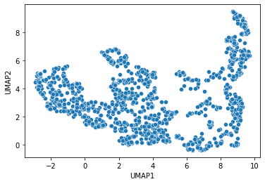
As the measured statistics are a large table with many columns, we cannot easily get a picture of the distribution of the data points. For a clustering algorithm it might also be challenging. Thus, we reduce the number of dimensions, e.g. using the Uniform Manifold Approximation Projection (UMAP).

reducer = umap.UMAP(random_state=42)
embedding = reducer.fit_transform(scaled_statistics)
type(embedding), embedding.shape

(numpy.ndarray, (1200, 2))

seaborn.scatterplot(x=embedding[:, 0], 
                    y=embedding[:, 1])

plt.xlabel('UMAP1')
plt.ylabel('UMAP2')

Text(0, 0.5, 'UMAP2')

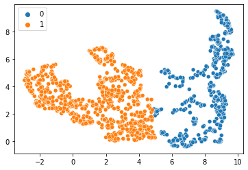
K-means clustering

Eventually, we will automatically annotate all data points with a class. In the following we will separate data points into two classes. Looking at the UMAP visualized above, we need an algorithm that takes relationsships of datapoints locally into account. K-means clustering has the capability to group data points in a way so that the distance between the data points to the cluster centers is minimal. It basically splits the data points along a region in the plot where the density of the data points is lower than in cluster centers, e.g. in the plot above where UMAP1 is approximately 5.

num_classes = 2

kmeans = KMeans(n_clusters=num_classes, random_state=42).fit(embedding)

kmeans_prediction = kmeans.predict(embedding)

C:\Users\rober\miniconda3\envs\bio_39\lib\site-packages\sklearn\cluster\_kmeans.py:1332: UserWarning: KMeans is known to have a memory leak on Windows with MKL, when there are less chunks than available threads. You can avoid it by setting the environment variable OMP_NUM_THREADS=5.
  warnings.warn(

seaborn.scatterplot(x=embedding[:, 0], 
                    y=embedding[:, 1],
                    hue=kmeans_prediction)

<AxesSubplot:>

We can also project the cluster identifier (0 or 1) back into the 3D image space. We just need to make sure we cannot mix up these two classes with background.

# suffix [0] represents background
# we add 1 to the measurement so that there is no 
# cluster with ID 0, which corresponds to background.
cluster_id = [0] + (kmeans_prediction + 1).tolist()

kmeans_prediction_map = cle.replace_intensities(nuclei_labels, cluster_id)

cle.imshow(kmeans_prediction_map, labels=True)

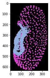
Interpreting clustering results

For technical reasons it is illegal to claim that k-means clustering can differentiate serosa and embryo. The algorithm was not informed about what to differentiate and thus, just differentiates objects according to their properties. It is now the task of the scientists to figure out which parameters influenced the decision making. For example, if shape-based parameters dominated the decision making, a follow-up questions would be why so. It might be possible that nuclei within the embryo are differently shaped than nuclei within the serosa. But it is also possible that the nuclei segmentation algorithm caused objects to be segmented wrongly. Thus, clustering is just a tool for generating new hypotheses which need to be investigated further, before an algorithm can be designed that differentiates nuclei in serosa and embryo. Such an algorithm then also needs to be validated, e.g. by processing new, unseen datasets, and measuring the quality of the clustering quantitatively, e.g. by providing ground-truth annotations and comparing with them.