Metrics to investigate segmentation quality

When we apply a segmentation algorithm to an image, we can ask for good reason how good the segmentation result is. Actually, a common problem is that checking and improving the quality of segmentation results is often omitted and done rather by the the appearance of the segmentation result than by actually quantifying it. So lets look at different ways to achieve this quantification.

from skimage.io import imread, imshow
import napari
from the_segmentation_game import metrics as metrics_game
import pyclesperanto_prototype as cle
import matplotlib.pyplot as plt
import numpy as np
import pandas as pd
from sklearn import metrics
from sklearn.metrics import PrecisionRecallDisplay

For this, we will explore a dataset of the marine annelid Platynereis dumerilii from Ozpolat, B. et al licensed by CC BY 4.0. We will concentrate on a single timepoint.

We already have ground truth (gt) annotations and segmentation result and are now just importing them.

gt = imread("../../data/Platynereis_tp7_channel1_rescaled(256x256x103)_gt.tif")
segmentation = imread("../../data/Platynereis_tp7_channel1_rescaled(256x256x103)_voronoi_otsu_label_image.tif")

For image visualization, we will use napari.

viewer = napari.Viewer()

WARNING: QWindowsWindow::setGeometry: Unable to set geometry 1086x680+1195+219 (frame: 1104x727+1186+181) on QWidgetWindow/"_QtMainWindowClassWindow" on "\\.\DISPLAY1". Resulting geometry: 905x925+1193+212 (frame: 923x972+1184+174) margins: 9, 38, 9, 9 minimum size: 374x575 MINMAXINFO maxSize=0,0 maxpos=0,0 mintrack=392,622 maxtrack=0,0)

Now we are adding gt and segmentation result as labels to our napari-viewer:

viewer.add_labels(gt, name = 'Ground truth')
viewer.add_labels(segmentation, name = 'Segmentation')

<Labels layer 'Segmentation' at 0x267db70ac40>

And change in the viewer from 2D to 3D view:

viewer.dims.ndisplay=3

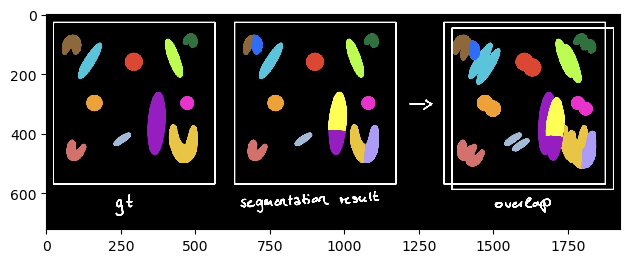
In gallery view, you can see on the left now our segmentation result and the right our gt:

napari.utils.nbscreenshot(viewer)

For determining the quality of a segmentation result, we need a metrics. There are different useful metrics:

Jaccard index

The Jaccard index is a measure to investigate the similarity or difference of sample sets

In the-segmentation-game, we can find 3 different implementations of the Jaccard index:

The sparse Jaccard Index measures the overlap lying between 0 (no overlap) and 1 (perfect overlap). Therefore, the ground truth label is compared to the most overlapping segmented label. This value is then averaged over all annotated objects (see schematics).

# Jaccard index sparse
print('Jaccard index sparse: %.3f' % metrics_game.jaccard_index_sparse(gt,segmentation))

Jaccard index sparse: 0.555

scheme_sparse = imread('schematics/Jaccard_index_sparse.jpg')
imshow(scheme_sparse)

<matplotlib.image.AxesImage at 0x26781ec4af0>

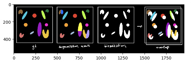
When using the binary Jaccard Index, gt and segmentation result are first binarized into foreground (= everything annotated) and background (= rest). Next, the overlap between the binary images is computed. This can be used for comparing binary segmentation results, e.g. thresholding techniques. However, when we try to compare our gt and segmentation, we get:

# Jaccard index binary
print('Jaccard index binary: %.3f' % metrics_game.jaccard_index_binary(gt,segmentation))

Jaccard index binary: 0.709

The binary Jaccard index is way higher than the sparse Jaccard index because the outline of individual labels is not taken into account. Only the outline between fore- and background plays a role (see schematics below):

scheme_binary = imread('schematics/Jaccard_index_binary.jpg')
imshow(scheme_binary)

<matplotlib.image.AxesImage at 0x26781f077c0>

So for cases like ours we should use the sparse Jaccard index and not the binary Jaccard index.

Terminology: What are TP, TN, FP, FN

We can also use different matrices which need true positives (TP), true negatives (TN), false positives (FP) and false negatives (FN).

We want to compute these for a segmentation result. Therefore, we are treating the segmentation result as a two class thresholding-problem. The two classes are forground and background. To make this clearer, we binarize the gt and the segmentation result:

threshold = 1
gt_binary = gt >= threshold
segmentation_binary = segmentation >= threshold

viewer.add_labels(gt_binary, name = 'Binary ground truth')
viewer.add_labels(segmentation_binary, name = 'Binary segmentation result')

<Labels layer 'Binary segmentation result' at 0x26781f3c7f0>

Now we have labels only consisting of foreground (1) and background (0) which we can nicely see in napari (gallery view):

napari.utils.nbscreenshot(viewer)

Now what are TP, TN, FP and FN?

• TP are pixels which are in gt and segmentation result foreground (1)

• TN are pixels which are in gt and segmentation result background (0)

• FP are pixels which are in gt background (0) but in the segmentation result foreground (1)

• FN are pixels which are in gt foreground (1) but in the segmentation result background (0)

Confusion matrix

These 4 can be nicely shown in a confusion matrix. Therefore, we will use scikit-learn (see also metrics documentation)

We now want to plot the confusion matrix of the binary images. To be able to use the confusion matrix, we need to turn our image into a 1-dimensional array like this:

gt_1d = np.ravel(gt_binary)
segmentation_1d = np.ravel(segmentation_binary)

confusion_matrix = metrics.confusion_matrix(gt_1d,segmentation_1d)

cm_display = metrics.ConfusionMatrixDisplay(confusion_matrix = confusion_matrix, display_labels = [False, True])

cm_display.plot()
plt.show()

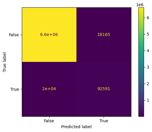
We can see that we mostly have TN which means that our image consist mostly of background.

Accuracy, Precision, Recall, F1-Score

Now we are computing metrics which are based on the concept of TP, TN, FP and FN.

Accuracy closely agrees with the accepted value. You basically ask: How well did my segmentation go regarding my two different classes (foreground and background)?

print('Accuracy: %.3f' % metrics.accuracy_score(gt_1d, segmentation_1d))
#In binary classification, this function is equal to the jaccard_score function

Accuracy: 0.994

This indicates that the segmentation algorithm performed correct in most instances.

Precision shows similarities between the measurements. You basically ask: How well did my segmentation go regarding the predicion of foreground objects?

print('Precision: %.3f' % metrics.precision_score(gt_1d, segmentation_1d))

Precision: 0.836

This means that FP were lowering down the precision score.

Recall is the true positive rate (TPR) aka Sensitivity. You basically ask: How many instances were correctly identified as foreground?

print('Recall: %.3f' % metrics.recall_score(gt_1d, segmentation_1d))

Recall: 0.823

This means that out of the positive class, the model did perform wel, but FN were lowering down the recall-score.

F1-Score is the harmonic mean between precision and recall score. You basically ask: Can I find a compromise when choosing between precision and recall score? This results in a trade-off between high false-positives and false-negative rates.

In our case, precision and recall were very similar which means it is not really needed to compute the F1-Score. If we compute it we get a similar outcome:

print('F1 Score: %.3f' % metrics.f1_score(gt_1d, segmentation_1d))

F1 Score: 0.830

Exercise

Now, we produce a gt and a segmentation result ourselves:

gt_new = np.array([[0, 1, 1],
               [0, 1, 0]])
segmentation_new = np.array([[0, 1, 0],
                       [0, 1, 1]])

fig, ax = plt.subplots(1,2)

ax[0].imshow(gt_new)
ax[0].set_title('gt')
ax[1].imshow(segmentation_new)
ax[1].set_title('segmentation result')

Text(0.5, 1.0, 'segmentation result')

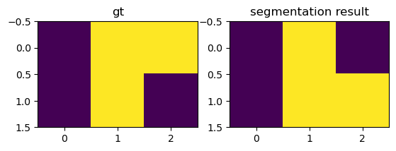
As you can see, they are binary images consisting out of 0 (dark blue) and 1 (yellow). Can you compute a confusion matrix for this example? Try it out and interpret the results you get!