Object classification with APOC and SimpleITK-based features#
Classifying objects can involve extracting custom features. We simulate this scenario by using SimpleITK-based features as available in napari-simpleitk-image-processing and train an APOC table-row-classifier.
See also
from skimage.io import imread
from pyclesperanto_prototype import imshow, replace_intensities
from skimage.filters import threshold_otsu
from skimage.measure import label, regionprops
import numpy as np
import pandas as pd
import matplotlib.pyplot as plt
from napari_simpleitk_image_processing import label_statistics
import apoc
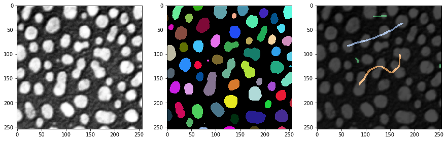
Our starting point are an image, a label image and some ground truth annotation. The annotation is also a label image where the user was just drawing lines with different intensity (class) through small objects, large objects and elongated objects.
# load and label data
image = imread('../../data/blobs.tif')
labels = label(image > threshold_otsu(image))
annotation = imread('../../data/label_annotation.tif')

# visualize
fig, ax = plt.subplots(1,3, figsize=(15,15))
imshow(image, plot=ax[0])
imshow(labels, plot=ax[1], labels=True)
imshow(image, plot=ax[2], continue_drawing=True)
imshow(annotation, plot=ax[2], alpha=0.7, labels=True)
Feature extraction#
The first step to classify objects according to their properties is feature extraction. We will use the scriptable napari plugin napari-simpleitk-image-processing for that.
statistics = label_statistics(image, labels, None, True, True, True, True, True, True)

statistics_table = pd.DataFrame(statistics)
statistics_table
| label | maximum | mean | median | minimum | sigma | sum | variance | bbox_0 | bbox_1 | ... | number_of_pixels_on_border | perimeter | perimeter_on_border | perimeter_on_border_ratio | principal_axes0 | principal_axes1 | principal_axes2 | principal_axes3 | principal_moments0 | principal_moments1 | |
|---|---|---|---|---|---|---|---|---|---|---|---|---|---|---|---|---|---|---|---|---|---|
| 0 | 1 | 232.0 | 190.854503 | 200.0 | 128.0 | 30.304925 | 82640.0 | 918.388504 | 10 | 0 | ... | 17 | 89.196525 | 17.0 | 0.190590 | 0.902586 | 0.430509 | -0.430509 | 0.902586 | 17.680049 | 76.376232 |
| 1 | 2 | 224.0 | 179.286486 | 184.0 | 128.0 | 21.883314 | 33168.0 | 478.879436 | 53 | 0 | ... | 21 | 53.456120 | 21.0 | 0.392846 | -0.051890 | -0.998653 | 0.998653 | -0.051890 | 8.708186 | 27.723954 |
| 2 | 3 | 248.0 | 205.617021 | 208.0 | 128.0 | 29.380812 | 135296.0 | 863.232099 | 95 | 0 | ... | 23 | 93.409370 | 23.0 | 0.246228 | 0.988608 | 0.150515 | -0.150515 | 0.988608 | 49.978765 | 57.049896 |
| 3 | 4 | 248.0 | 217.327189 | 232.0 | 128.0 | 36.061134 | 94320.0 | 1300.405402 | 144 | 0 | ... | 19 | 75.558902 | 19.0 | 0.251459 | 0.870813 | 0.491615 | -0.491615 | 0.870813 | 33.246984 | 37.624111 |
| 4 | 5 | 248.0 | 212.142558 | 224.0 | 128.0 | 29.904270 | 101192.0 | 894.265349 | 237 | 0 | ... | 39 | 82.127941 | 40.0 | 0.487045 | 0.998987 | 0.045005 | -0.045005 | 0.998987 | 24.584386 | 60.694273 |
| ... | ... | ... | ... | ... | ... | ... | ... | ... | ... | ... | ... | ... | ... | ... | ... | ... | ... | ... | ... | ... | ... |
| 59 | 60 | 128.0 | 128.000000 | 128.0 | 128.0 | 0.000000 | 128.0 | 0.000000 | 110 | 246 | ... | 0 | 2.681517 | 0.0 | 0.000000 | 1.000000 | 0.000000 | 0.000000 | 1.000000 | 0.000000 | 0.000000 |
| 60 | 61 | 248.0 | 183.407407 | 176.0 | 128.0 | 34.682048 | 14856.0 | 1202.844444 | 170 | 248 | ... | 19 | 41.294008 | 19.0 | 0.460115 | -0.005203 | -0.999986 | 0.999986 | -0.005203 | 2.190911 | 21.525901 |
| 61 | 62 | 216.0 | 181.511111 | 184.0 | 128.0 | 25.599001 | 16336.0 | 655.308864 | 116 | 249 | ... | 23 | 48.093086 | 23.0 | 0.478239 | -0.023708 | -0.999719 | 0.999719 | -0.023708 | 1.801689 | 31.523372 |
| 62 | 63 | 248.0 | 188.377358 | 184.0 | 128.0 | 38.799398 | 9984.0 | 1505.393324 | 227 | 249 | ... | 16 | 34.264893 | 16.0 | 0.466950 | 0.004852 | -0.999988 | 0.999988 | 0.004852 | 1.603845 | 13.711214 |
| 63 | 64 | 224.0 | 172.897959 | 176.0 | 128.0 | 28.743293 | 8472.0 | 826.176871 | 66 | 250 | ... | 17 | 35.375614 | 17.0 | 0.480557 | 0.022491 | -0.999747 | 0.999747 | 0.022491 | 0.923304 | 18.334505 |
64 rows × 33 columns
statistics_table.columns
Index(['label', 'maximum', 'mean', 'median', 'minimum', 'sigma', 'sum',
       'variance', 'bbox_0', 'bbox_1', 'bbox_2', 'bbox_3', 'centroid_0',
       'centroid_1', 'elongation', 'feret_diameter', 'flatness', 'roundness',
       'equivalent_ellipsoid_diameter_0', 'equivalent_ellipsoid_diameter_1',
       'equivalent_spherical_perimeter', 'equivalent_spherical_radius',
       'number_of_pixels', 'number_of_pixels_on_border', 'perimeter',
       'perimeter_on_border', 'perimeter_on_border_ratio', 'principal_axes0',
       'principal_axes1', 'principal_axes2', 'principal_axes3',
       'principal_moments0', 'principal_moments1'],
      dtype='object')
table = statistics_table[['number_of_pixels','elongation']]
table
| number_of_pixels | elongation | |
|---|---|---|
| 0 | 433 | 2.078439 |
| 1 | 185 | 1.784283 |
| 2 | 658 | 1.068402 |
| 3 | 434 | 1.063793 |
| 4 | 477 | 1.571246 |
| ... | ... | ... |
| 59 | 1 | 0.000000 |
| 60 | 81 | 3.134500 |
| 61 | 90 | 4.182889 |
| 62 | 53 | 2.923862 |
| 63 | 49 | 4.456175 |
64 rows × 2 columns
We also read out the maximum intensity of every labeled object from the ground truth annotation. These values will serve to train the classifier. Entries of 0 correspond to objects that have not been annotated.
annotation_stats = regionprops(labels, intensity_image=annotation)

annotated_classes = np.asarray([s.max_intensity for s in annotation_stats])
print(annotated_classes)
[0. 0. 2. 0. 0. 0. 2. 0. 0. 0. 3. 0. 0. 0. 3. 0. 0. 3. 0. 0. 0. 3. 0. 0.
 0. 0. 1. 0. 0. 0. 1. 2. 1. 0. 0. 2. 0. 1. 0. 0. 0. 0. 0. 0. 0. 0. 0. 0.
 0. 0. 0. 0. 0. 0. 0. 0. 0. 0. 0. 0. 0. 0. 0. 0.]
Classifier Training#
Next, we can train the Random Forest Classifer. It needs tablue training data and a ground truth vector.
classifier_filename = 'table_row_classifier.cl'

classifier = apoc.TableRowClassifier(opencl_filename=classifier_filename, max_depth=2, num_ensembles=10)
classifier.train(table, annotated_classes)
Prediction#
To apply a classifier to the whole dataset, or any other dataset, we need to make sure that the data is in the same format. This is trivial in case we analyse the same dataset we trained on.
predicted_classes = classifier.predict(table)
predicted_classes
array([1, 1, 2, 3, 3, 3, 2, 3, 2, 1, 3, 3, 3, 2, 3, 1, 3, 3, 3, 3, 3, 3,
       1, 3, 3, 3, 3, 1, 3, 3, 1, 2, 1, 2, 2, 3, 3, 1, 1, 3, 3, 3, 3, 2,
       3, 2, 3, 2, 1, 3, 1, 3, 3, 1, 3, 3, 3, 3, 1, 2, 1, 1, 1, 1],
      dtype=uint32)
For documentation purposes, we can save the annotated class and the predicted class into the our table. Note: We’re doing this after training, because otherwise e.g. the column
table
| number_of_pixels | elongation | |
|---|---|---|
| 0 | 433 | 2.078439 |
| 1 | 185 | 1.784283 |
| 2 | 658 | 1.068402 |
| 3 | 434 | 1.063793 |
| 4 | 477 | 1.571246 |
| ... | ... | ... |
| 59 | 1 | 0.000000 |
| 60 | 81 | 3.134500 |
| 61 | 90 | 4.182889 |
| 62 | 53 | 2.923862 |
| 63 | 49 | 4.456175 |
64 rows × 2 columns
table['annotated_class'] = annotated_classes
table['predicted_class'] = predicted_classes
table
/var/folders/p1/6svzckgd1y5906pfgm71fvmr0000gn/T/ipykernel_4463/2818530951.py:1: SettingWithCopyWarning:
A value is trying to be set on a copy of a slice from a DataFrame.
Try using .loc[row_indexer,col_indexer] = value instead

See the caveats in the documentation: https://pandas.pydata.org/pandas-docs/stable/user_guide/indexing.html#returning-a-view-versus-a-copy
  table['annotated_class'] = annotated_classes
/var/folders/p1/6svzckgd1y5906pfgm71fvmr0000gn/T/ipykernel_4463/2818530951.py:2: SettingWithCopyWarning:
A value is trying to be set on a copy of a slice from a DataFrame.
Try using .loc[row_indexer,col_indexer] = value instead

See the caveats in the documentation: https://pandas.pydata.org/pandas-docs/stable/user_guide/indexing.html#returning-a-view-versus-a-copy
  table['predicted_class'] = predicted_classes
| number_of_pixels | elongation | annotated_class | predicted_class | |
|---|---|---|---|---|
| 0 | 433 | 2.078439 | 0.0 | 1 |
| 1 | 185 | 1.784283 | 0.0 | 1 |
| 2 | 658 | 1.068402 | 2.0 | 2 |
| 3 | 434 | 1.063793 | 0.0 | 3 |
| 4 | 477 | 1.571246 | 0.0 | 3 |
| ... | ... | ... | ... | ... |
| 59 | 1 | 0.000000 | 0.0 | 2 |
| 60 | 81 | 3.134500 | 0.0 | 1 |
| 61 | 90 | 4.182889 | 0.0 | 1 |
| 62 | 53 | 2.923862 | 0.0 | 1 |
| 63 | 49 | 4.456175 | 0.0 | 1 |
64 rows × 4 columns
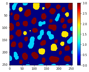
Furthermore, we can use the same vector to use replace_intensities to generate a class_image. The background and objects with NaNs in measurements will have value 0 in that image.
# we add a 0 for the class of background at the beginning
predicted_classes_with_background = [0] + predicted_classes.tolist()
print(predicted_classes_with_background)
[0, 1, 1, 2, 3, 3, 3, 2, 3, 2, 1, 3, 3, 3, 2, 3, 1, 3, 3, 3, 3, 3, 3, 1, 3, 3, 3, 3, 1, 3, 3, 1, 2, 1, 2, 2, 3, 3, 1, 1, 3, 3, 3, 3, 2, 3, 2, 3, 2, 1, 3, 1, 3, 3, 1, 3, 3, 3, 3, 1, 2, 1, 1, 1, 1]
class_image = replace_intensities(labels, predicted_classes_with_background)
imshow(class_image, colorbar=True, colormap='jet', min_display_intensity=0)