Slicing and cropping#
When working with larger image data, it often makes sense to crop out regions and focus on them for further analysis. For cropping images, we use the same “:”-syntax, we used when indexing in lists and exploring multi-dimensional image data.
import numpy as np
from skimage.io import imread, imshow
We start by loading a 3D image and printing its size.
image = imread("../../data/Haase_MRT_tfl3d1.tif")

image.shape
(192, 256, 256)
Slicing#
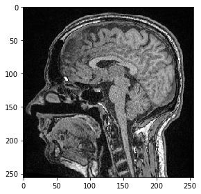
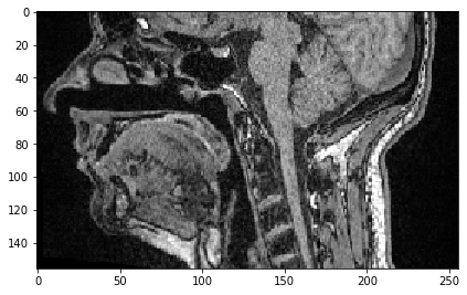
For visualizing 3D images using scikit-image’s imshow, we need to select a slice to visualize. For example, a Z-slice:
slice_image = image[100]

imshow(slice_image)
<matplotlib.image.AxesImage at 0x2b54f73d340>
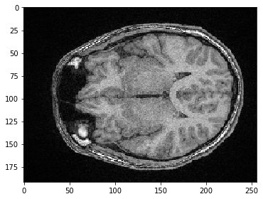
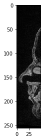
We can also select a plane where all pixels have the same Y-position. We just need to specify, that we would like to keep all pixels in Z using the : syntax.
slice_image = image[:, 100]

imshow(slice_image)
<matplotlib.image.AxesImage at 0x2b54f836af0>
Cropping#
We can also select a sub-stack using indexing in the square brackets.
sub_stack = image[50:150]

sub_stack.shape
(100, 256, 256)
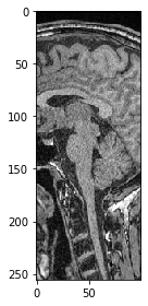
We can also select a sub-region in X. If we want to keep all pixels along Z and Y (the first two dimensions), we just specify : to keep all.
sub_region_x = image[:, :, 100:200]

imshow(sub_region_x[100])
<matplotlib.image.AxesImage at 0x2b54f8ae850>
For selectinng all pixels in one direction above a given value, we just need to specify the start before :.
sub_region_y = image[:, 100:]

imshow(sub_region_y[100])
<matplotlib.image.AxesImage at 0x2b54f90ae20>
Similarly, we can select all pixels up to a given position.
sub_region_x2 = image[:, :, :50]

imshow(sub_region_x2[100])
<matplotlib.image.AxesImage at 0x2b550943d30>
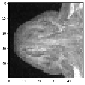
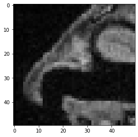
Last but not least, this is how a cropped cube is specified.
cropped_cube = image[80:130, 120:170, :50]

cropped_cube.shape
(50, 50, 50)
imshow(cropped_cube[20])
<matplotlib.image.AxesImage at 0x2b5509a4a00>
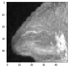
And this is how a maximum-intensity projections of this cropped cube look like.
maximum_intensity_projection_along_z = np.max(cropped_cube, axis=0)
imshow(maximum_intensity_projection_along_z)
<matplotlib.image.AxesImage at 0x2b550a03f40>
maximum_intensity_projection_along_y = np.max(cropped_cube, axis=1)
imshow(maximum_intensity_projection_along_y)
<matplotlib.image.AxesImage at 0x2b550a5e8e0>