Supervised machine learning

Supervised machine learning is a technique for configuring (learning) parameters of a computational model based on annotated data. In this example, we provide sparsely annotated data, which means we only annotate some of the given data points.

See also

• Supervised learning (Wikipedia)

• Supervised learning in scikit-learn

import matplotlib.pyplot as plt
import pandas as pd
from sklearn.ensemble import RandomForestClassifier
from sklearn.metrics import jaccard_score, accuracy_score, precision_score, recall_score

# local import; this library is located in the same folder as the notebook
from data_generator import generate_biomodal_2d_data

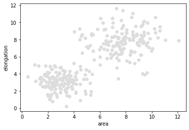
Our starting point for demonstrating supervised machine learning is a a pair of measurements in a bimodal distribution. In the following data set objects with a larger area are typically also more elongated.

data = generate_biomodal_2d_data()

plt.scatter(data[:, 0], data[:, 1], c='#DDDDDD')
plt.xlabel('area')
plt.ylabel('elongation')

Text(0, 0.5, 'elongation')

To get a more detailed insight into the data, we print out the first entries.

data_to_annotate = data[:20]

pd.DataFrame(data_to_annotate, columns=["area", "elongation"])

	area	elongation
0	3.950088	2.848643
1	4.955912	3.390093
2	7.469852	5.575289
3	2.544467	3.017479
4	3.465662	1.463756
5	3.156507	3.232181
6	9.978705	6.676372
7	6.001683	5.047063
8	2.457139	3.416050
9	3.672295	3.407462
10	9.413702	7.598608
11	2.896781	3.410599
12	2.305432	2.850365
13	4.640594	8.602249
14	3.523277	2.828454
15	7.636970	10.277392
16	7.223721	6.531755
17	7.146032	8.404857
18	7.407157	6.260869
19	6.543343	8.472226

Annotating data

As mentioned above, supervised machine learning algorithms need some form of annotation, also called ground truth. We create a list of annotations where 1 represents small objects and 2 represents large and elongated objects.

Note: We are here annotating the first 20 data points, which is a quite small number. In real projects, larger amounts of annotation data might be necessary to train well-performing classifiers.

manual_annotation = [1, 1, 2, 1, 1, 1, 2, 2, 1, 1, 2, 1, 1, 2, 1, 2, 2, 2, 2, 2]

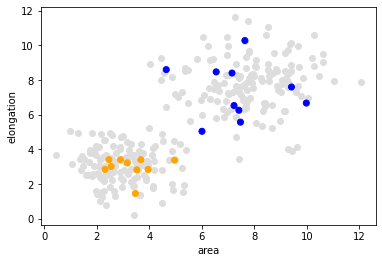
Now, we visualize the measurements again and draw the annotated measurements on top.

plt.scatter(data[:, 0], data[:, 1], c='#DDDDDD')
plt.xlabel('area')
plt.ylabel('elongation')

colors = ['orange', 'blue']
annotated_colors = [colors[i-1] for i in manual_annotation]

plt.scatter(data_to_annotate[:, 0], data_to_annotate[:, 1], c=annotated_colors)

<matplotlib.collections.PathCollection at 0x14d8ee3d790>

Separating test and validation data

Before we train our classifier, we need to split the annotated data into two subsets. Goal is to enable unbiased validation. We train on the first half of the annotated data points and measure the quality on the second half. Read more.

train_data = data_to_annotate[:10]
validation_data = data_to_annotate[10:]

train_annotation = manual_annotation[:10]
validation_annotation = manual_annotation[10:]

Classifier training

With the selected data to annotate and the manual annotation, we can train a Random Forest Classifier.

classifier = RandomForestClassifier()
classifier.fit(train_data, train_annotation)

RandomForestClassifier()

Validation

We can now apply the classifier to the validation data and measure how many of these data points have been analyzed correctly.

result = classifier.predict(validation_data)

# Show results next to annotation in a table
result_annotation_comparison_table = {
    "Predicted": result,
    "Annotated": validation_annotation
}
pd.DataFrame(result_annotation_comparison_table)

	Predicted	Annotated
0	2	2
1	1	1
2	1	1
3	1	2
4	1	1
5	2	2
6	2	2
7	2	2
8	2	2
9	2	2

To get some standardized measures of the quality of the results of our classifier, we use scikit-learn’s metrics. An overview about the techniques are also available on Wikipedia and mean in the context here:

• Accurcay: What portion of predictions were correct?

• Precision: What portion of predicted 1s were annotated as 1?

• Recall (sensitivity): What portion of predicted 2s have been annotated as 2?

accuracy_score(validation_annotation, result)

0.9

precision_score(validation_annotation, result)

0.75

recall_score(validation_annotation, result)

1.0

If you want to understand more detailed how the enties are counted and the quality scores are computed, the multilabel confusion matrix may be worth a look.

Prediction

After training and validation of the classifier, we can reuse it to process other data sets. It is uncommon to classify test- and validation data, as those should be used for making the classifier only. We here apply the classifier to the remaining data points, which have not been annotated.

remaining_data = data[20:]

prediction = classifier.predict(remaining_data)
prediction

array([1, 1, 1, 1, 2, 1, 2, 1, 2, 1, 2, 2, 1, 2, 2, 1, 1, 2, 1, 1, 1, 1,
       2, 1, 2, 2, 2, 2, 2, 1, 1, 1, 2, 1, 2, 1, 2, 1, 2, 1, 2, 1, 1, 2,
       2, 2, 1, 1, 1, 1, 1, 2, 1, 1, 2, 2, 2, 1, 1, 2, 2, 1, 2, 2, 2, 1,
       1, 1, 1, 1, 2, 1, 2, 1, 2, 1, 2, 2, 1, 2, 1, 1, 2, 1, 1, 1, 1, 2,
       1, 2, 1, 2, 2, 1, 1, 2, 2, 2, 2, 2, 2, 1, 2, 2, 1, 1, 1, 2, 2, 2,
       1, 2, 2, 2, 1, 2, 1, 2, 2, 1, 2, 2, 1, 1, 2, 1, 1, 2, 1, 2, 1, 1,
       1, 1, 1, 1, 2, 1, 1, 1, 1, 2, 1, 1, 2, 2, 2, 1, 1, 1, 1, 2, 2, 1,
       1, 1, 1, 2, 2, 1, 2, 1, 1, 2, 2, 1, 1, 2, 1, 2, 1, 2, 1, 2, 2, 2,
       1, 2, 1, 2, 1, 1, 2, 2, 2, 1, 1, 1, 2, 1, 2, 2, 1, 2, 1, 2, 1, 1,
       2, 1, 1, 2, 1, 1, 2, 2, 2, 1, 1, 1, 2, 2, 2, 2, 2, 1, 2, 1, 1, 2,
       2, 2, 1, 1, 2, 1, 1, 2, 1, 2, 2, 2, 1, 1, 2, 2, 1, 1, 1, 2, 2, 1,
       1, 1, 1, 1, 2, 2, 1, 1, 1, 1, 1, 1, 2, 2, 2, 1, 1, 2, 2, 2, 1, 2,
       1, 2, 2, 1, 2, 2, 1, 2, 2, 1, 1, 2, 1, 1, 2, 1])

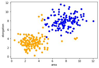
Here we now visualize the whole data set with class colors.

predicted_colors = [colors[i-1] for i in prediction]

plt.scatter(remaining_data[:, 0], remaining_data[:, 1], c=predicted_colors)
plt.xlabel('area')
plt.ylabel('elongation')

Text(0, 0.5, 'elongation')

Exercise

Train a Support Vector Machine and visualize its prediction.

from sklearn.svm import SVC

classifier = SVC()