Surface measurements#
In this notebook we demonstrate how to retrieve surface/vertex measurements in a table and how to visualize them on the surface. The used example data is derived from AV Luque and JV Veenvliet (2023) licensed CC-BY. See the creating_surfaces notebook for how to create the surface from raw imaging data.
See also
import napari
import matplotlib.pyplot as plt
from napari.utils import nbscreenshot
import numpy as np
import vedo
from napari_process_points_and_surfaces import add_curvature, Curvature, spherefitted_curvature
import napari_process_points_and_surfaces as nppas

import vedo
viewer = napari.Viewer(ndisplay=3)
viewer.camera.angles = (40, -30, 55)
surface = nppas.gastruloid()
The nppas gastruloid example is derived from AV Luque and JV Veenvliet (2023) which is licensed CC-BY (https://creativecommons.org/licenses/by/4.0/legalcode) and can be downloaded from here: https://zenodo.org/record/7603081
Surface visualization#
The surface itself does not come with any quantification. It looks like this:
surface

|
nppas.SurfaceTuple
|
Quantification#
We can create a table (pandas Dataframe) like this.
requested_measurements = [nppas.Quality.AREA,
                          nppas.Quality.ASPECT_RATIO,
                          nppas.Quality.GAUSS_CURVATURE,
                          nppas.Quality.MEAN_CURVATURE,
                          nppas.Quality.SPHERE_FITTED_CURVATURE_DECA_VOXEL,
                          nppas.Quality.SPHERE_FITTED_CURVATURE_HECTA_VOXEL,
                          nppas.Quality.SPHERE_FITTED_CURVATURE_KILO_VOXEL,
                         ]

df = nppas.surface_quality_table(surface, requested_measurements)
df
| vertex_index | Quality.AREA | Quality.ASPECT_RATIO | Quality.GAUSS_CURVATURE | Quality.MEAN_CURVATURE | Quality.SPHERE_FITTED_CURVATURE_DECA_VOXEL | Quality.SPHERE_FITTED_CURVATURE_HECTA_VOXEL | Quality.SPHERE_FITTED_CURVATURE_KILO_VOXEL | |
|---|---|---|---|---|---|---|---|---|
| 0 | 0 | 29.997389 | 1.600400 | 0.030287 | 0.000490 | 0.000691 | 0.000257 | 0.000019 |
| 1 | 1 | 46.087046 | 1.602183 | 0.011136 | 0.000018 | NaN | 0.000250 | 0.000019 |
| 2 | 2 | 35.886338 | 1.400599 | 0.012633 | 0.000142 | 0.000542 | 0.000253 | 0.000019 |
| 3 | 3 | 22.887296 | 1.751932 | 0.036979 | 0.000548 | 0.000339 | 0.000379 | 0.000019 |
| 4 | 4 | 29.952347 | 1.220882 | 0.010277 | 0.000047 | 0.000366 | 0.000391 | 0.000019 |
| ... | ... | ... | ... | ... | ... | ... | ... | ... |
| 3319 | 3319 | 25.079661 | 1.340802 | 0.031878 | 0.000606 | 0.001081 | 0.000168 | 0.000019 |
| 3320 | 3320 | 47.213916 | 1.254924 | 0.004615 | 0.000003 | NaN | 0.000169 | 0.000019 |
| 3321 | 3321 | 35.964707 | 1.140267 | 0.015661 | 0.000198 | 0.000547 | 0.000163 | 0.000019 |
| 3322 | 3322 | 45.673529 | 1.189562 | 0.011380 | 0.000100 | 0.000026 | 0.000152 | 0.000019 |
| 3323 | 3323 | 30.105530 | 1.151230 | 0.014396 | 0.000190 | 0.000158 | 0.000163 | 0.000019 |
3324 rows × 8 columns
To get an overview about measurements, we can summarize them:
df.describe().T
| count | mean | std | min | 25% | 50% | 75% | max | |
|---|---|---|---|---|---|---|---|---|
| vertex_index | 3324.0 | 1661.500000 | 959.700474 | 0.000000e+00 | 830.750000 | 1661.500000 | 2492.250000 | 3323.000000 |
| Quality.AREA | 3324.0 | 33.753233 | 10.790780 | 5.677486e+00 | 26.694735 | 32.956835 | 39.255080 | 125.564101 |
| Quality.ASPECT_RATIO | 3324.0 | 7.126810 | 89.909602 | 1.038034e+00 | 1.292444 | 1.437911 | 1.648299 | 3421.965459 |
| Quality.GAUSS_CURVATURE | 3324.0 | 0.016958 | 0.035275 | -1.031106e+00 | 0.005509 | 0.013645 | 0.024739 | 0.348243 |
| Quality.MEAN_CURVATURE | 3324.0 | 0.000383 | 0.007653 | -2.803460e-02 | -0.000135 | 0.000010 | 0.000270 | 0.426018 |
| Quality.SPHERE_FITTED_CURVATURE_DECA_VOXEL | 2750.0 | 0.002875 | 0.004761 | 1.791201e-09 | 0.000341 | 0.001004 | 0.003054 | 0.043508 |
| Quality.SPHERE_FITTED_CURVATURE_HECTA_VOXEL | 3324.0 | 0.000258 | 0.000069 | 1.516446e-04 | 0.000214 | 0.000241 | 0.000275 | 0.000545 |
| Quality.SPHERE_FITTED_CURVATURE_KILO_VOXEL | 3324.0 | 0.000019 | 0.000000 | 1.853513e-05 | 0.000019 | 0.000019 | 0.000019 | 0.000019 |
We can extract a single column for the table as list.
curvature = list(df['Quality.SPHERE_FITTED_CURVATURE_HECTA_VOXEL'])
curvature[:5]
[0.0002572409502622459,
 0.0002504286604301336,
 0.00025319922419934937,
 0.00037887302369609083,
 0.00039058361737075804]
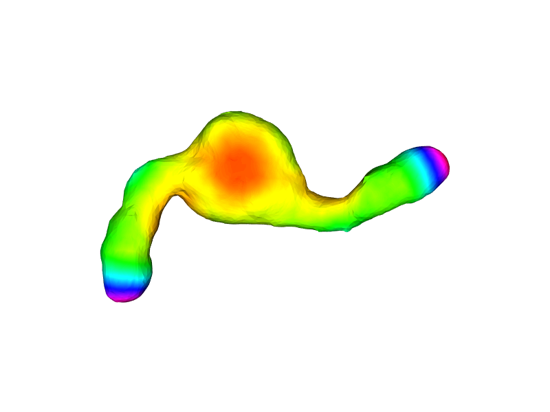
Visualizing measurements#
To visualize the measurements, we need to attach them to the surface:
quantified_surface = nppas.set_vertex_values(surface, curvature)
quantified_surface

|
nppas.SurfaceTuple

|
The visualization can be customized as well, e.g. by changing the view angle and the colormap.
nppas.show(quantified_surface, azimuth=-90, cmap='jet')
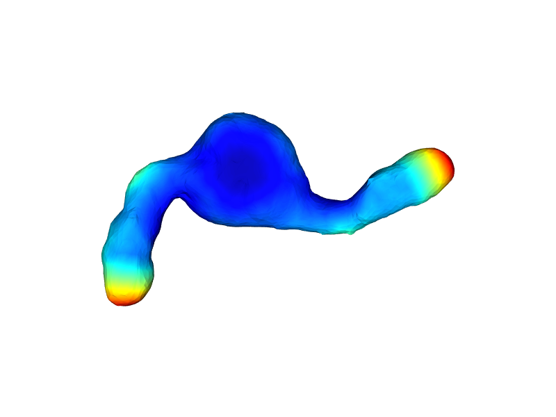
nppas.show(quantified_surface, azimuth=-90, cmap='hsv')