Post-processing binary images using morphological operations

Morphological operations transform images based on shape; typically we mean binary images in this context.

import numpy as np
from skimage.io import imread
import matplotlib.pyplot as plt
from skimage import morphology
from skimage import filters

Kernels, footsprints and structural elements

If we work with scikit-image, many morphological filters have a footprint parameter. This footprint is the filter kernel, and in the literature you also find the term structural element for this.

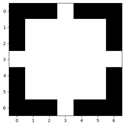
# creates a disk of 1 with radius = 3
disk = morphology.disk(3) 
disk

array([[0, 0, 0, 1, 0, 0, 0],
       [0, 1, 1, 1, 1, 1, 0],
       [0, 1, 1, 1, 1, 1, 0],
       [1, 1, 1, 1, 1, 1, 1],
       [0, 1, 1, 1, 1, 1, 0],
       [0, 1, 1, 1, 1, 1, 0],
       [0, 0, 0, 1, 0, 0, 0]], dtype=uint8)

plt.imshow(disk, cmap='gray')

<matplotlib.image.AxesImage at 0x225b0c88340>

# create a square with width and height = 3
square = morphology.square(3) 
square

array([[1, 1, 1],
       [1, 1, 1],
       [1, 1, 1]], dtype=uint8)

Binary morphology

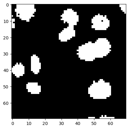
For demonstrating morphological filtering of binary images, we use the small nuclei image again.

image_nuclei = imread('../../data/mitosis_mod.tif').astype(float)
image_binary = image_nuclei > filters.threshold_otsu(image_nuclei)

plt.imshow(image_binary, cmap='gray')

<matplotlib.image.AxesImage at 0x225b0d05490>

Erosion and Dilation

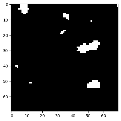
To make white islands in the black ocean smaller, we need to erode its coastlines.

eroded = morphology.binary_erosion(image_binary, disk)

plt.imshow(eroded, cmap='gray')

<matplotlib.image.AxesImage at 0x225b0d80dc0>

If we dilate the image afterwards, we get white islands back that look smoother than in the original binary image.

eroded_dilated = morphology.binary_dilation(eroded, disk)

plt.imshow(eroded_dilated, cmap='gray')

<matplotlib.image.AxesImage at 0x225b107f730>

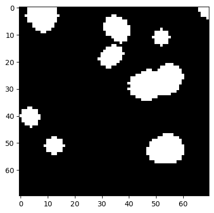
Calling erosion and dilation subsequently is so common that there is an extra function which does exactly that. As the gab between islands open the operation is called opening.

opened = morphology.binary_opening(image_binary, disk)

plt.imshow(opened, cmap='gray')

<matplotlib.image.AxesImage at 0x225b10f9b20>

Exercise 1

There is also a closing operation. Apply it to the binary image.

Exercise 2

Search the scikit-image documentation for minimum and maximum filters. Apply the minimum filter to the binary image and the maximum filter to the result afterwards. Compare it to the images shown above.