Inspecting 3D image data with pyclesperanto

This notebook demonstrates how to navigate through 3D images.

import pyclesperanto_prototype as cle

import numpy as np
import matplotlib
import matplotlib.pyplot as plt
from skimage.io import imread

# Laod example data
input_image = imread('../../data/Haase_MRT_tfl3d1.tif')

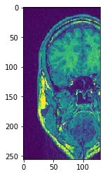
Copy Slice

In order to visualize crop specific slices; without the image leaving GPU memory, use the copy_slice method.

# Copy Slice
image_slice = cle.create([256, 256]);
slice_z_position = 40.0;
cle.copy_slice(input_image, image_slice, slice_z_position)

# show result
cle.imshow(image_slice)

# Alternatively, don't hand over the output image and retrieve it
another_slice = cle.create_2d_xy(input_image)
cle.copy_slice(input_image, another_slice, slice_index = 80)

# show result
cle.imshow(another_slice)

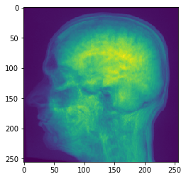
Projection

pyclesperanto offers min/mean/max and sum projections in x, y and z.

# Maximum Z Projection
projection = cle.maximum_z_projection(input_image)

# show result
cle.imshow(projection)

If you pass an image stack to cle.imshow it will make the maximum intensity projection along Z for you:

cle.imshow(input_image)

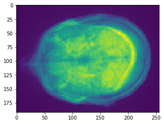
# Sum Z Projection
projection = cle.sum_z_projection(input_image)

# show result
cle.imshow(projection)

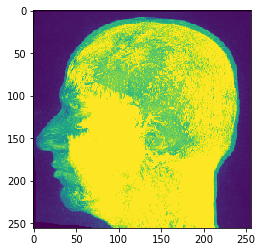
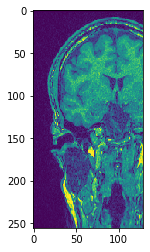
# Mean Y Projection
projection = cle.mean_y_projection(input_image)

# show result
cle.imshow(projection)

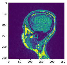
Transpose XZ

In order to transpose axes of images in the GPU, use the transpose methods

# Transpose X against Z
transposed_image = cle.create([256, 256, 129]);
cle.transpose_xz(input_image, transposed_image)

# show result
cle.imshow(transposed_image[126])
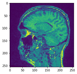
cle.imshow(transposed_image[98])

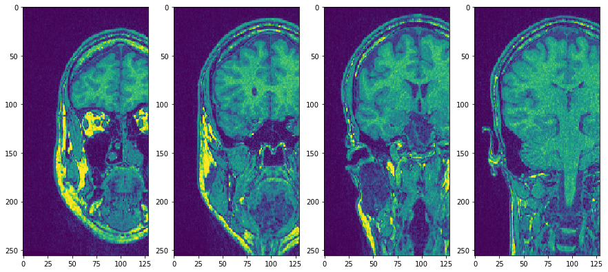
Use subplots to but them side by side

fig, axs = plt.subplots(1, 4, figsize=(15, 7))
cle.imshow(transposed_image[75], plot=axs[0])
cle.imshow(transposed_image[100], plot=axs[1])
cle.imshow(transposed_image[125], plot=axs[2])
cle.imshow(transposed_image[150], plot=axs[3])