Opening LIF files#
When working with microscopy image data, many file formats are circulating such as the Leica Image Format (LIF). In this notebook, we will open a .lif file using the readlif library.
Note: It is recommended to use AICSImageIO for reading LIF images as shown in this notebook.
The readlif library can be installed like this from the terminal:
pip install readlif
After installing it, it can be imported.
from readlif.reader import LifFile

import os
import requests
from skimage.io import imshow
import numpy as np
As example dataset, we will use an image shared by Gregory Marquart and Harold Burgess under CC-BY 4.0 license. We need to download it first.
filename = "../../data/y293-Gal4_vmat-GFP-f01.lif"
url = 'https://zenodo.org/record/3382102/files/y293-Gal4_vmat-GFP-f01.lif?download=1'

if not os.path.isfile(filename):
    # only download the file if we don't have it yet
    response = requests.get(url)
    open(filename, "wb").write(response.content)
At this point the file should be on our computer and can be opened like this.
file = LifFile(filename)
file
'LifFile object with 1 image'
lif_image = file.get_image(0)
lif_image
'LifImage object with dimensions: Dims(x=616, y=500, z=86, t=1, m=1)'
From the LifImage, we can get individual frames as PIL images.
pil_image = lif_image.get_frame(z=0)
type(pil_image)
PIL.Image.Image
Finally, these 2D PIL images can be converted into numpy arrays. Which allows us eventually to take a look at the image.
np_image = np.array(pil_image)
np_image.shape
(500, 616)
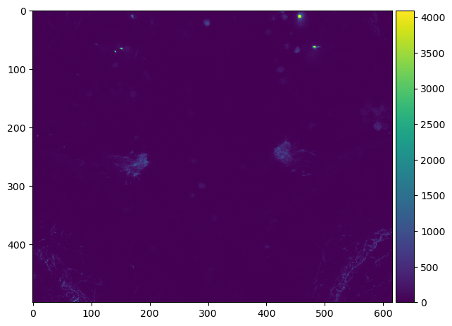
imshow(np_image)
/opt/miniconda3/envs/devbio-napari-env/lib/python3.9/site-packages/skimage/io/_plugins/matplotlib_plugin.py:149: UserWarning: Low image data range; displaying image with stretched contrast.
  lo, hi, cmap = _get_display_range(image)
<matplotlib.image.AxesImage at 0x1378ab970>
To access all pixels in our 3D image, we should first have a look in the metadata of the file.
lif_image.info
{'dims': Dims(x=616, y=500, z=86, t=1, m=1),
 'display_dims': (1, 2),
 'dims_n': {1: 616, 2: 500, 3: 86},
 'scale_n': {1: 2.1354804344851965,
  2: 2.135480168493237,
  3: 0.9929687300128537},
 'path': 'Experiment_002/',
 'name': 'Series011',
 'channels': 2,
 'scale': (2.1354804344851965, 2.135480168493237, 0.9929687300128537, None),
 'bit_depth': (12, 12),
 'mosaic_position': [],
 'channel_as_second_dim': False,
 'settings': {}}
For example, it might be useful later to know the voxel size in z/y/x order.
voxel_size = lif_image.info['scale'][2::-1]
voxel_size
(0.9929687300128537, 2.135480168493237, 2.1354804344851965)
We can also read out how many slices the 3D stack has.
num_slices = lif_image.info['dims'].z
num_slices
86
This information allows us to write a convenience function that allows converting the LIF image into a 3D numpy image stack.
def lif_to_numpy_stack(lif_image):
    num_slices = lif_image.info['dims'].z

    return np.asarray([np.array(lif_image.get_frame(z=z)) for z in range(num_slices)])
image_stack = lif_to_numpy_stack(lif_image)
image_stack.shape
(86, 500, 616)
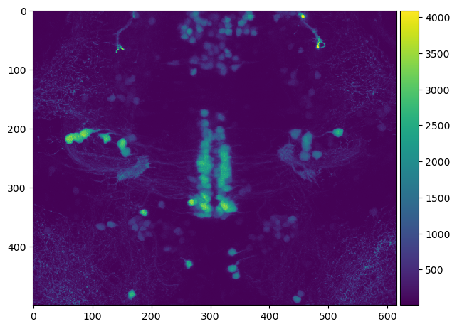
This image stack can then be used for example to visualize a maximum intensity projection along Z.
imshow(np.max(image_stack, axis=0))
<matplotlib.image.AxesImage at 0x137a1c610>