Probability maps#
APOC is based on pyclesperanto and sklearn.
Let’s start with loading an example image and some ground truth:
from skimage.io import imread, imshow, imsave
import matplotlib.pyplot as plt
import numpy as np
import apoc
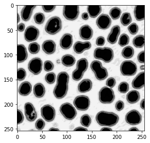
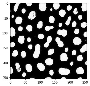
image = imread('blobs.tif')
imshow(image)
<matplotlib.image.AxesImage at 0x25fc553f9a0>
do_manual_annotation = False
if do_manual_annotation: # you can use this to make manual annotations
import napari
# start napari
viewer = napari.Viewer()
napari.run()
# add image
viewer.add_image(image)
# add an empty labels layer and keep it in a variable
labels = np.zeros(image.shape).astype(int)
viewer.add_labels(labels)
else:
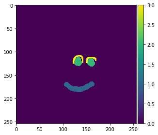
labels = imread('annotations_3class.tif')
manual_annotations = labels
if do_manual_annotation:
    imsave('annotations_3class.tif', manual_annotations)

from skimage.io import imshow
imshow(manual_annotations, vmin=0, vmax=3)
C:\Users\rober\miniconda3\envs\bio_38\lib\site-packages\skimage\io\_plugins\matplotlib_plugin.py:150: UserWarning: Low image data range; displaying image with stretched contrast.
  lo, hi, cmap = _get_display_range(image)
<matplotlib.image.AxesImage at 0x25fc565c5e0>
Training#
We now train a PixelClassifier, which is under the hood a scikit-learn RandomForestClassifier. After training, the classifier will be converted to clij-compatible OpenCL code and save to disk under a given filename.
# define features: original image, a blurred version and an edge image
features = "original gaussian_blur=2 sobel_of_gaussian_blur=2"

# this is where the model will be saved
cl_filename = 'my_model.cl'

output_probability_of_class = 3

apoc.erase_classifier(cl_filename)
clf = apoc.ProbabilityMapper(opencl_filename=cl_filename, output_probability_of_class=output_probability_of_class)
clf.train(features, manual_annotations, image)
Prediction#
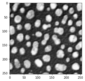
The classifier can then be used to classify all pixels in the given image. Starting point is again, the feature stack. Thus, the user must make sure that the same features are used for training and for prediction.
result = clf.predict(image=image)
imshow(result)
<matplotlib.image.AxesImage at 0x25fc5770670>
Training / prediction for other classes#
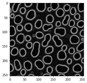
We will now train again and output the probability of another class
output_probability_of_class = 2

apoc.erase_classifier(cl_filename)
clf = apoc.ProbabilityMapper(opencl_filename=cl_filename, output_probability_of_class=output_probability_of_class)
clf.train(features, manual_annotations, image)

result = clf.predict(image=image)
imshow(result)
<matplotlib.image.AxesImage at 0x25fc57d9d30>
output_probability_of_class = 1

apoc.erase_classifier(cl_filename)
clf = apoc.ProbabilityMapper(opencl_filename=cl_filename, output_probability_of_class=output_probability_of_class)
clf.train(features, manual_annotations, image)

result = clf.predict(image=image)
imshow(result)
<matplotlib.image.AxesImage at 0x25fc58484c0>