Pixel classification using Scikit-learn#
Pixel classification is a technique for assigning pixels to multiple classes. If there are two classes (object and background), we are talking about binarization. In this example we use a random forest classifier for pixel classification.
See also
from sklearn.ensemble import RandomForestClassifier

from skimage.io import imread, imshow
import numpy as np
import napari
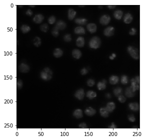
As example image, use the image set BBBC038v1, available from the Broad Bioimage Benchmark Collection Caicedo et al., Nature Methods, 2019.
image = imread('../../data/BBBC038/0bf4b1.tif')

imshow(image)
<matplotlib.image.AxesImage at 0x7f817af51ac0>
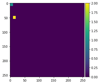
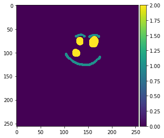
For demonstrating how the algorithm works, we annotate two small regions on the left of the image with values 1 and 2 for background and foreground (objects).
annotation = np.zeros(image.shape)
annotation[0:10,0:10] = 1
annotation[45:55,10:20] = 2

imshow(annotation, vmin=0, vmax=2)
/Users/haase/opt/anaconda3/envs/bio_39/lib/python3.9/site-packages/skimage/io/_plugins/matplotlib_plugin.py:150: UserWarning: Low image data range; displaying image with stretched contrast.
  lo, hi, cmap = _get_display_range(image)
/Users/haase/opt/anaconda3/envs/bio_39/lib/python3.9/site-packages/skimage/io/_plugins/matplotlib_plugin.py:150: UserWarning: Float image out of standard range; displaying image with stretched contrast.
  lo, hi, cmap = _get_display_range(image)
<matplotlib.image.AxesImage at 0x7f81180937c0>
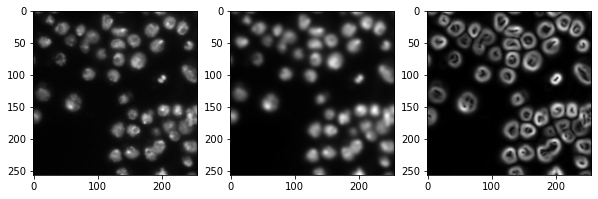
Generating a feature stack#
Pixel classifiers such as the random forest classifier takes multiple images as input. We typically call these images a feature stack because for every pixel exist now multiple values (features). In the following example we create a feature stack containing three features:
The original pixel value
The pixel value after a Gaussian blur
The pixel value of the Gaussian blurred image processed through a Sobel operator.
Thus, we denoise the image and detect edges. All three images serve the pixel classifier to differentiate positive and negative pixels.
from skimage import filters

def generate_feature_stack(image):
    # determine features
    blurred = filters.gaussian(image, sigma=2)
    edges = filters.sobel(blurred)

    # collect features in a stack
    # The ravel() function turns a nD image into a 1-D image.
    # We need to use it because scikit-learn expects values in a 1-D format here.
    feature_stack = [
        image.ravel(),
        blurred.ravel(),
        edges.ravel()
    ]

    # return stack as numpy-array
    return np.asarray(feature_stack)

feature_stack = generate_feature_stack(image)

# show feature images
import matplotlib.pyplot as plt
fig, axes = plt.subplots(1, 3, figsize=(10,10))

# reshape(image.shape) is the opposite of ravel() here. We just need it for visualization.
axes[0].imshow(feature_stack[0].reshape(image.shape), cmap=plt.cm.gray)
axes[1].imshow(feature_stack[1].reshape(image.shape), cmap=plt.cm.gray)
axes[2].imshow(feature_stack[2].reshape(image.shape), cmap=plt.cm.gray)
<matplotlib.image.AxesImage at 0x7f817b16d5e0>
Formatting data#
We now need to format the input data so that it fits to what scikit learn expects. Scikit-learn asks for an array of shape (n, m) as input data and (n) annotations. n corresponds to number of pixels and m to number of features. In our case m = 3.
def format_data(feature_stack, annotation):
    # reformat the data to match what scikit-learn expects
    # transpose the feature stack
    X = feature_stack.T
    # make the annotation 1-dimensional
    y = annotation.ravel()

    # remove all pixels from the feature and annotations which have not been annotated
    mask = y > 0
    X = X[mask]
    y = y[mask]

    return X, y

X, y = format_data(feature_stack, annotation)

print("input shape", X.shape)
print("annotation shape", y.shape)
input shape (200, 3)
annotation shape (200,)
Training the random forest classifier#
We now train the random forest classifier by providing the feature stack X and the annotations y.
classifier = RandomForestClassifier(max_depth=2, random_state=0)
classifier.fit(X, y)
RandomForestClassifier(max_depth=2, random_state=0)
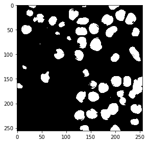
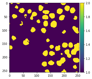
Predicting pixel classes#
After the classifier has been trained, we can use it to predict pixel classes for whole images. Note in the following code, we provide feature_stack.T which are more pixels then X in the commands above, because it also contains the pixels which were not annotated before.
res = classifier.predict(feature_stack.T) - 1 # we subtract 1 to make background = 0
imshow(res.reshape(image.shape))
<matplotlib.image.AxesImage at 0x7f817b59fd90>
Interactive segmentation#
We can also use napari to annotate some regions as negative (label = 1) and positive (label = 2).
# start napari
viewer = napari.Viewer()

# add image
viewer.add_image(image)

# add an empty labels layer and keet it in a variable
labels = viewer.add_labels(np.zeros(image.shape).astype(int))
/Users/haase/opt/anaconda3/envs/bio_39/lib/python3.9/site-packages/napari_tools_menu/__init__.py:165: FutureWarning: Public access to Window.qt_viewer is deprecated and will be removed in
v0.5.0. It is considered an "implementation detail" of the napari
application, not part of the napari viewer model. If your use case
requires access to qt_viewer, please open an issue to discuss.
  self.tools_menu = ToolsMenu(self, self.qt_viewer.viewer)
Go ahead after annotating at least two regions with labels 1 and 2.
Take a screenshot of the annotation:
napari.utils.nbscreenshot(viewer)

Retrieve the annotations from the napari layer:
manual_annotations = labels.data

imshow(manual_annotations, vmin=0, vmax=2)
/Users/haase/opt/anaconda3/envs/bio_39/lib/python3.9/site-packages/skimage/io/_plugins/matplotlib_plugin.py:150: UserWarning: Low image data range; displaying image with stretched contrast.
  lo, hi, cmap = _get_display_range(image)
<matplotlib.image.AxesImage at 0x7f8158e05a30>
As we have used functions in the example above, we can just repeat the same procedure with the manual annotations.
# generate features (that's actually not necessary,
# as the variable is still there and the image is the same.
# but we do it for completeness)
feature_stack = generate_feature_stack(image)
X, y = format_data(feature_stack, manual_annotations)

# train classifier
classifier = RandomForestClassifier(max_depth=2, random_state=0)
classifier.fit(X, y)

# process the whole image and show result
result_1d = classifier.predict(feature_stack.T)
result_2d = result_1d.reshape(image.shape)
imshow(result_2d)
/Users/haase/opt/anaconda3/envs/bio_39/lib/python3.9/site-packages/skimage/io/_plugins/matplotlib_plugin.py:150: UserWarning: Low image data range; displaying image with stretched contrast.
  lo, hi, cmap = _get_display_range(image)
<matplotlib.image.AxesImage at 0x7f8138dea5e0>
Also we add the result to napari.
viewer.add_labels(result_2d)
<Labels layer 'result_2d' at 0x7f816a1faaf0>
napari.utils.nbscreenshot(viewer)

Exercise#
Change the code so that you can annotate three different regions:
Nuclei
Background
The edges between blobs and background