Statistics using SimpleITK#
We can use SimpleITK for extracting features from label images. For convenience reasons we use the napari-simpleitk-image-processing library.
import numpy as np
import pandas as pd
from skimage.io import imread
from pyclesperanto_prototype import imshow
from skimage import measure
import pyclesperanto_prototype as cle
from skimage import filters
from napari_simpleitk_image_processing import label_statistics
# load image
image = imread("../../data/blobs.tif")
# denoising
blurred_image = filters.gaussian(image, sigma=1)
# binarization
threshold = filters.threshold_otsu(blurred_image)
thresholded_image = blurred_image >= threshold
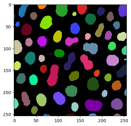
# labeling
label_image = measure.label(thresholded_image)
# visualization
imshow(label_image, labels=True)
Measurements/ region properties#
We are now using the very handy function label_statistics which provides a table of features. Let us check first what we need to provide for this function:
label_statistics?
Signature:
label_statistics(
intensity_image: 'napari.types.ImageData',
label_image: 'napari.types.LabelsData',
size: bool = True,
intensity: bool = True,
perimeter: bool = False,
shape: bool = False,
position: bool = False,
moments: bool = False,
napari_viewer: 'napari.Viewer' = None,
) -> 'pandas.DataFrame'
Docstring:
Measure intensity/shape/... statistics per label
Parameters
----------
intensity_image: ndarray, optional
Can be None
label_image: ndarray
Must be subsequently labeled
size: bool, optional
intensity: bool, optional
perimeter: bool, optional
shape: bool, optional
position: bool, optional
moments: bool, optional
napari_viewer: napari.Viewer, optional
Returns
-------
pandas DataFrame, in case napari_viewr is None, otherwise the DataFrame will be added to
the passed label_image's layer.features
See Also
--------
..[0] https://simpleitk.org/doxygen/latest/html/classitk_1_1simple_1_1LabelShapeStatisticsImageFilter
..[1] http://insightsoftwareconsortium.github.io/SimpleITK-Notebooks/Python_html/35_Segmentation_Shape_Analysis.html
File: c:\users\maral\mambaforge\envs\feature_blogpost\lib\site-packages\napari_simpleitk_image_processing\_simpleitk_image_processing.py
Type: function
Feature categories which are set to True are measured by default. In this case, the categories are size and intensity. But the rest might be also interesting to investigate. So we need to set them to True as well:
df = pd.DataFrame(label_statistics(image, label_image,
shape=True,
perimeter=True,
position=True,
moments=True))
df
| label | maximum | mean | median | minimum | sigma | sum | variance | bbox_0 | bbox_1 | ... | number_of_pixels_on_border | perimeter | perimeter_on_border | perimeter_on_border_ratio | principal_axes0 | principal_axes1 | principal_axes2 | principal_axes3 | principal_moments0 | principal_moments1 | |
|---|---|---|---|---|---|---|---|---|---|---|---|---|---|---|---|---|---|---|---|---|---|
| 0 | 1 | 232.0 | 191.440559 | 200.0 | 128.0 | 29.827923 | 82128.0 | 889.704987 | 10 | 0 | ... | 16 | 87.070368 | 16.0 | 0.183759 | 0.905569 | 0.424199 | -0.424199 | 0.905569 | 17.336255 | 75.599678 |
| 1 | 2 | 224.0 | 179.846995 | 184.0 | 128.0 | 21.328889 | 32912.0 | 454.921516 | 53 | 0 | ... | 21 | 53.456120 | 21.0 | 0.392846 | -0.042759 | -0.999085 | 0.999085 | -0.042759 | 8.637199 | 27.432794 |
| 2 | 3 | 248.0 | 205.604863 | 208.0 | 120.0 | 29.414615 | 135288.0 | 865.219581 | 95 | 0 | ... | 23 | 93.409370 | 23.0 | 0.246228 | 0.989650 | 0.143505 | -0.143505 | 0.989650 | 49.994764 | 56.996778 |
| 3 | 4 | 248.0 | 217.515012 | 232.0 | 120.0 | 35.893817 | 94184.0 | 1288.366094 | 144 | 0 | ... | 20 | 76.114262 | 20.0 | 0.262763 | 0.902854 | 0.429947 | -0.429947 | 0.902854 | 33.290649 | 37.542552 |
| 4 | 5 | 248.0 | 213.033898 | 224.0 | 128.0 | 28.771575 | 100552.0 | 827.803519 | 237 | 0 | ... | 39 | 82.127941 | 40.0 | 0.487045 | 0.999090 | 0.042642 | -0.042642 | 0.999090 | 24.209327 | 60.391416 |
| ... | ... | ... | ... | ... | ... | ... | ... | ... | ... | ... | ... | ... | ... | ... | ... | ... | ... | ... | ... | ... | ... |
| 57 | 58 | 224.0 | 184.525822 | 192.0 | 120.0 | 28.322029 | 39304.0 | 802.137302 | 39 | 232 | ... | 0 | 52.250114 | 0.0 | 0.000000 | 0.976281 | 0.216509 | -0.216509 | 0.976281 | 13.084485 | 21.981750 |
| 58 | 59 | 248.0 | 184.810127 | 184.0 | 128.0 | 33.955505 | 14600.0 | 1152.976306 | 170 | 248 | ... | 18 | 39.953250 | 18.0 | 0.450527 | -0.012197 | -0.999926 | 0.999926 | -0.012197 | 2.075392 | 20.902016 |
| 59 | 60 | 216.0 | 182.727273 | 184.0 | 128.0 | 24.557101 | 16080.0 | 603.051202 | 117 | 249 | ... | 22 | 46.196967 | 22.0 | 0.476222 | -0.014920 | -0.999889 | 0.999889 | -0.014920 | 1.815666 | 29.359308 |
| 60 | 61 | 248.0 | 189.538462 | 192.0 | 128.0 | 38.236858 | 9856.0 | 1462.057315 | 227 | 249 | ... | 15 | 32.924135 | 15.0 | 0.455593 | -0.013675 | -0.999906 | 0.999906 | -0.013675 | 1.592570 | 12.843450 |
| 61 | 62 | 224.0 | 173.833333 | 176.0 | 128.0 | 28.283770 | 8344.0 | 799.971631 | 66 | 250 | ... | 17 | 35.375614 | 17.0 | 0.480557 | 0.030675 | -0.999529 | 0.999529 | 0.030675 | 0.917610 | 17.904873 |
62 rows × 33 columns
These are all columns that are available:
print(df.keys())
Index(['label', 'maximum', 'mean', 'median', 'minimum', 'sigma', 'sum',
'variance', 'bbox_0', 'bbox_1', 'bbox_2', 'bbox_3', 'centroid_0',
'centroid_1', 'elongation', 'feret_diameter', 'flatness', 'roundness',
'equivalent_ellipsoid_diameter_0', 'equivalent_ellipsoid_diameter_1',
'equivalent_spherical_perimeter', 'equivalent_spherical_radius',
'number_of_pixels', 'number_of_pixels_on_border', 'perimeter',
'perimeter_on_border', 'perimeter_on_border_ratio', 'principal_axes0',
'principal_axes1', 'principal_axes2', 'principal_axes3',
'principal_moments0', 'principal_moments1'],
dtype='object')
df.describe()
| label | maximum | mean | median | minimum | sigma | sum | variance | bbox_0 | bbox_1 | ... | number_of_pixels_on_border | perimeter | perimeter_on_border | perimeter_on_border_ratio | principal_axes0 | principal_axes1 | principal_axes2 | principal_axes3 | principal_moments0 | principal_moments1 | |
|---|---|---|---|---|---|---|---|---|---|---|---|---|---|---|---|---|---|---|---|---|---|
| count | 62.000000 | 62.000000 | 62.000000 | 62.000000 | 62.000000 | 62.000000 | 62.000000 | 62.000000 | 62.000000 | 62.000000 | ... | 62.000000 | 62.000000 | 62.000000 | 62.000000 | 62.000000 | 62.000000 | 62.000000 | 62.000000 | 62.000000 | 62.000000 |
| mean | 31.500000 | 233.548387 | 190.429888 | 196.258065 | 125.161290 | 28.767558 | 69534.451613 | 864.079980 | 121.532258 | 112.629032 | ... | 5.564516 | 67.071263 | 5.580645 | 0.102864 | 0.703539 | -0.114112 | 0.114112 | 0.703539 | 20.742486 | 43.535735 |
| std | 18.041619 | 19.371838 | 15.382559 | 19.527144 | 4.602898 | 6.091478 | 42911.182492 | 311.860596 | 80.574925 | 76.921129 | ... | 9.667625 | 23.507575 | 9.724986 | 0.173858 | 0.459158 | 0.537821 | 0.537821 | 0.459158 | 13.092549 | 32.666912 |
| min | 1.000000 | 152.000000 | 146.285714 | 144.000000 | 112.000000 | 6.047432 | 1024.000000 | 36.571429 | 0.000000 | 0.000000 | ... | 0.000000 | 9.155272 | 0.000000 | 0.000000 | -0.651619 | -0.999926 | -0.660963 | -0.651619 | 0.489796 | 0.571429 |
| 25% | 16.250000 | 232.000000 | 182.969505 | 186.000000 | 120.000000 | 26.561523 | 36010.000000 | 705.524752 | 53.000000 | 43.250000 | ... | 0.000000 | 52.551616 | 0.000000 | 0.000000 | 0.752633 | -0.624188 | -0.318631 | 0.752633 | 11.068721 | 22.027192 |
| 50% | 31.500000 | 240.000000 | 190.749492 | 200.000000 | 128.000000 | 29.089645 | 71148.000000 | 846.217207 | 121.000000 | 110.500000 | ... | 0.000000 | 68.204464 | 0.000000 | 0.000000 | 0.937869 | 0.040942 | -0.040942 | 0.937869 | 18.744728 | 35.367902 |
| 75% | 46.750000 | 248.000000 | 199.725305 | 208.000000 | 128.000000 | 32.583571 | 99962.000000 | 1061.691674 | 197.250000 | 172.250000 | ... | 12.500000 | 84.307520 | 12.500000 | 0.184963 | 0.994807 | 0.318631 | 0.624188 | 0.994807 | 29.519182 | 56.938641 |
| max | 62.000000 | 248.000000 | 220.026144 | 240.000000 | 136.000000 | 38.374793 | 177944.000000 | 1472.624704 | 251.000000 | 250.000000 | ... | 39.000000 | 125.912897 | 40.000000 | 0.487045 | 1.000000 | 0.660963 | 0.999926 | 1.000000 | 49.994764 | 186.225041 |
8 rows × 33 columns
Specific measures#
SimpleITK offers some non-standard measurements which deserve additional documentation
number_of_pixels_on_border#
First, we check its range on the above example image.
number_of_pixels_on_border = df['number_of_pixels_on_border'].tolist()
np.min(number_of_pixels_on_border), np.max(number_of_pixels_on_border)
(0, 39)
Next, we visualize the measurement in space.
number_of_pixels_on_border_map = cle.replace_intensities(label_image, [0] + number_of_pixels_on_border)
number_of_pixels_on_border_map

|
cle._ image

|
The visualization suggests that number_of_pixels_on_border is the count of pixels within a label that is located at the image border.
perimeter_on_border#
perimeter_on_border = df['perimeter_on_border'].tolist()
np.min(perimeter_on_border), np.max(perimeter_on_border)
perimeter_on_border_map = cle.replace_intensities(label_image, [0] + perimeter_on_border)
perimeter_on_border_map

|
cle._ image

|
The visualization suggests that perimeter_on_border is the perimeter of labels that are located at the image border.
perimeter_on_border_ratio#
In this context, the SimpleITK documentation points to a publication which mentiones “‘SizeOnBorder’ is the number of pixels in the objects which are on the border of the image.” While the documentation is wage, the perimeter_on_border_ratio may be related.
perimeter_on_border_ratio = df['perimeter_on_border_ratio'].tolist()
np.min(perimeter_on_border_ratio), np.max(perimeter_on_border_ratio)
perimeter_on_border_ratio_map = cle.replace_intensities(label_image, [0] + perimeter_on_border_ratio)
perimeter_on_border_ratio_map

|
cle._ image

|
The visualization reinforces our assumption that the perimeter_on_border_ratio indeed is related to the amount the object touches the image border.
principal axes#
In our example, we have principal_axes0 - principal_axes3
principal_axes_0 = df['principal_axes0'].tolist()
np.min(principal_axes_0), np.max(principal_axes_0)
principal_axes_0_map = cle.replace_intensities(label_image, [0] + principal_axes_0)
principal_axes_0_map

|
cle._ image

|
(principal_axes3 looks the same)
principal_axes_1 = df['principal_axes1'].tolist()
np.min(principal_axes_1), np.max(principal_axes_1)
principal_axes_1_map = cle.replace_intensities(label_image, [0] + principal_axes_1)
principal_axes_1_map

|
cle._ image

|
principal_axes_2 = df['principal_axes2'].tolist()
np.min(principal_axes_2), np.max(principal_axes_2)
principal_axes_2_map = cle.replace_intensities(label_image, [0] + principal_axes_2)
principal_axes_2_map

|
cle._ image

|
principal moments#
principal_moments_0 = df['principal_moments0'].tolist()
np.min(principal_moments_0), np.max(principal_moments_0)

principal_moments_0_map = cle.replace_intensities(label_image, [0] + principal_moments_0)
principal_moments_0_map

|
cle._ image

|
principal_moments_1 = df['principal_moments1'].tolist()
np.min(principal_moments_1), np.max(principal_moments_1)

principal_moments_1_map = cle.replace_intensities(label_image, [0] + principal_moments_1)
principal_moments_1_map

|
cle._ image

|