Working with images

To do image data analysis, we first need to be able to do a few essential operations:

• opening images

• displaying images

• have a look at pixel statistics

See also

• Lecture notes on scikit image by Emmanuelle Gouillart

• Histograms of images

Opening images

Most images with standard extensions (tif, png etc.) can be read using the skimage.io.imread function. In case your image doesn’t you should consult the documentation of the given file format.

To use imread you have three possibilities:

• use the absolute path to an image file e.g. imread('/Users/username/Desktop/blobs.tif')

• use a relative path to where you currently are (you cand find out using the pwd command in a cell) i.e. imread('../../data/blobs.tif')

• use a url that points to an image file, for example from the GitHub repository imread('https://github.com/haesleinhuepf/BioImageAnalysisNotebooks/raw/main/data/blobs.tif')

Here we use a relative path. Respective to the current notebook, the data are two folder levels higher (../../) in a folder called data:

from skimage.io import imread

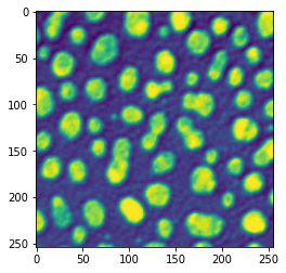
image = imread("../../data/blobs.tif")

As shown earlier, images are just matrices of intensities. However, showing them as such is not convenient.

image

array([[ 40,  32,  24, ..., 216, 200, 200],
       [ 56,  40,  24, ..., 232, 216, 216],
       [ 64,  48,  24, ..., 240, 232, 232],
       ...,
       [ 72,  80,  80, ...,  48,  48,  48],
       [ 80,  80,  80, ...,  48,  48,  48],
       [ 96,  88,  80, ...,  48,  48,  48]], dtype=uint8)

Displaying images

There are many ways to display simple 2D images. In many notebooks and examples online, you will find examples using Matplotlib’s imshow function on an array:

from matplotlib import pyplot as plt

plt.imshow(image);

Unfortunately, the imshow function is not an optimal choice to display microscopy images: it doesn’t handle well multi-channel data, it is difficult to handle intensity ranges etc. Throughout this course we therefore favor the use of the microshow function from the microfilm package or the imshow function from the clesperanto package. We’ll learn about the second solution in coming chapters. Here we just use microshow:

from microfilm.microplot import microshow

microshow(image);

Lookup tables (a.k.a. color maps)

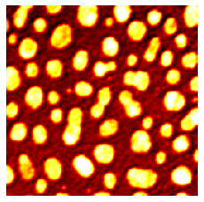
We can also change the look-up table, a.k.a. “color map” for the visualization.

microshow(image, cmaps="hot");

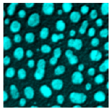
microshow(image, cmaps="pure_cyan");

Exercise

Open the banana020.tif data set, visualize it in a yellowish lookup table.