Measuring intensity on label borders#
In some applications it is reasonable to measure the intensity on label borders. For example, to measure the signal intensity in an image showing the nuclear envelope, one can segment nuclei, identify their borders and then measure the intensity there.
import numpy as np
from skimage.io import imread, imshow
import pyclesperanto_prototype as cle
from cellpose import models, io
from skimage import measure
import matplotlib.pyplot as plt
2022-02-24 10:05:10,405 [INFO] WRITING LOG OUTPUT TO C:\Users\rober\.cellpose\run.log
The example dataset#
In this example we load an image showing a zebrafish eye, courtesy of Mauricio Rocha Martins, Norden lab, MPI CBG Dresden.
multichannel_image = imread("../../data/zfish_eye.tif")
multichannel_image.shape
(1024, 1024, 3)
cropped_image = multichannel_image[200:600, 500:900]
nuclei_channel = cropped_image[:,:,0]

cle.imshow(nuclei_channel)
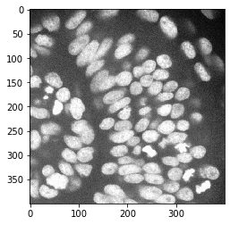
Image segmentation#
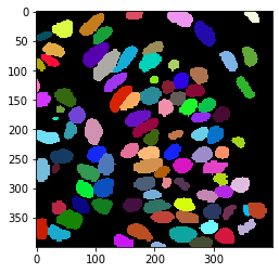
First, we use cellpose to segment the cells
# load cellpose model
model = models.Cellpose(gpu=False, model_type='nuclei')

# apply model
channels = [0,0] # This means we are processing single channel greyscale images.
label_image, flows, styles, diams = model.eval(nuclei_channel, diameter=None, channels=channels)

# show result
cle.imshow(label_image, labels=True)
2022-02-24 10:05:10,623 [INFO] >>>> using CPU
2022-02-24 10:05:10,675 [INFO] ~~~ ESTIMATING CELL DIAMETER(S) ~~~
2022-02-24 10:05:13,858 [INFO] estimated cell diameter(s) in 3.18 sec
2022-02-24 10:05:13,859 [INFO] >>> diameter(s) =
2022-02-24 10:05:13,860 [INFO] [ 29.64 ]
2022-02-24 10:05:13,860 [INFO] ~~~ FINDING MASKS ~~~
2022-02-24 10:05:18,649 [INFO] >>>> TOTAL TIME 7.97 sec
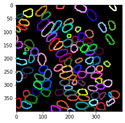
Labeling pixels on label borders#
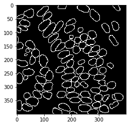
Next, we will extract the outline of the segmented nuclei.
binary_borders = cle.detect_label_edges(label_image)
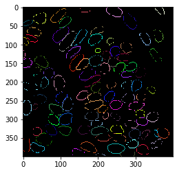
labeled_borders = binary_borders * label_image
cle.imshow(label_image, labels=True)
cle.imshow(binary_borders)
cle.imshow(labeled_borders, labels=True)
Dilating outlines#
We extend the outlines a bit to have a more robust measurement.
extended_outlines = cle.dilate_labels(labeled_borders, radius=2)

cle.imshow(extended_outlines, labels=True)
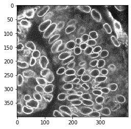
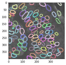
Overlay visualization#
Using this label image of nuclei outlines, we can measure the intensity in the nuclear envelope.
nuclear_envelope_channel = cropped_image[:,:,2]

cle.imshow(nuclear_envelope_channel)

cle.imshow(nuclear_envelope_channel, alpha=0.5, continue_drawing=True)
cle.imshow(extended_outlines, alpha=0.5, labels=True)
Label intensity statistics#
Measuring the intensity in the image works using the right intensty and label images.
stats = cle.statistics_of_labelled_pixels(nuclear_envelope_channel, extended_outlines)

stats["mean_intensity"]
array([35529.4  , 32835.07 , 36713.887, 37146.348, 49462.39 , 36392.6  ,
       37998.375, 48974.945, 31805.87 , 50451.793, 41006.047, 50854.016,
       36167.547, 41332.32 , 37815.766, 35121.38 , 43859.945, 40292.875,
       31583.992, 38933.57 , 32297.547, 39140.766, 37072.31 , 45990.57 ,
       39800.613, 37804.99 , 39092.43 , 39510.848, 40534.81 , 42057.293,
       44815.844, 42855.754, 38408.246, 41257.594, 37996.895, 38568.465,
       42331.266, 34748.973, 44219.844, 41986.086, 38606.215, 39008.094,
       36411.05 , 48155.797, 43781.97 , 38315.12 , 36048.39 , 37739.277,
       46268.816, 35808.32 , 37388.312, 37682.21 , 42932.72 , 38168.293,
       40489.73 , 43073.066, 40973.285, 40975.246, 39292.848, 38555.766,
       38219.785, 40054.242, 37356.87 , 45014.8  , 37211.668, 47025.47 ,
       30218.678, 33988.027, 37338.41 , 38500.85 , 38546.777, 40611.742,
       40391.453, 41024.46 , 37840.246, 41342.793, 39329.625, 43311.016,
       37829.074, 39949.82 , 39316.496, 40966.48 , 34066.7  , 34929.863,
       40356.445, 31959.607, 39480.855, 39194.027, 46274.582, 31316.648,
       37623.61 , 40962.016, 39203.37 , 45368.703, 37830.832, 35296.93 ,
       37756.1  , 39108.93 , 40739.543], dtype=float32)
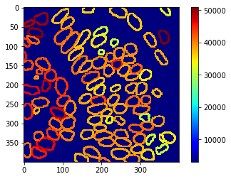
Parametric maps#
These measurements can also be visualized using parametric maps
intensity_map = cle.mean_intensity_map(nuclear_envelope_channel, extended_outlines)
cle.imshow(intensity_map, min_display_intensity=3000, colorbar=True, colormap="jet")
Exercise#
Measure and visualizae the intensity at the label borders in the nuclei channel.