Multidimensional image stacks#
Multi-dimensionsal image data data can be handled in a similar way as multi-channel image data.
Three-dimensional image stacks#
There are also images with three spatial dimensions: X, Y, and Z. You find typical examples in microscopy and in medical imaging. Let’s take a look at an Magnetic Resonance Imaging (MRI) data set:
from skimage.io import imread
from pyclesperanto_prototype import imshow
image_stack = imread('../../data/Haase_MRT_tfl3d1.tif')
image_stack.shape
(192, 256, 256)
We see that the data has indeed three dimensions, in this case 192 Z-planes and 256 X and Y pixels. We can display it with pyclesperanto’s imshow:
imshow(image_stack)
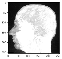
This MRI dataset looks unusal, because we are looking at a maximum intensity projection which is pyclesperanto’s default way of visualizing three-dimensional data.
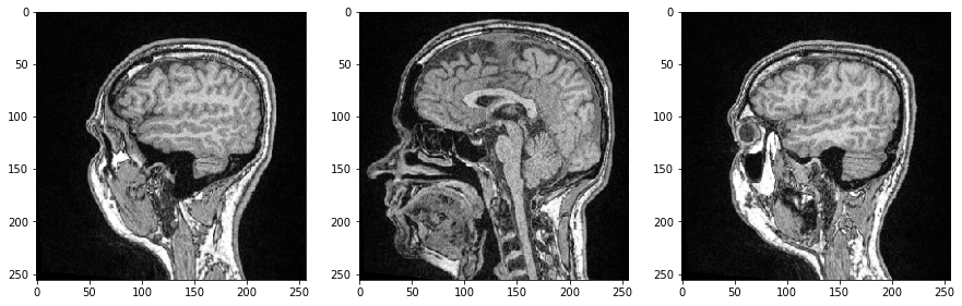
Image slicing#
We can inspect individual image slices by specifying their index in our 3D numpy array and this time use Matplotlib’s imshow for visualization:
import matplotlib.pyplot as plt
fig, axs = plt.subplots(1, 3, figsize=(15,15))

# show three planar images
axs[0].imshow(image_stack[48], cmap='Greys_r')
axs[1].imshow(image_stack[96], cmap='Greys_r')
axs[2].imshow(image_stack[144], cmap='Greys_r');
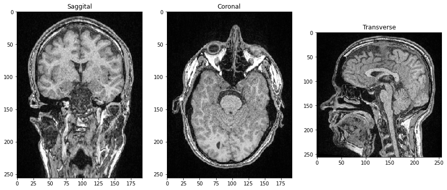
As all three dimensions are spatial dimensions, we can also make slices orthogonal to the image plane and corresponding to Anatomical planes. To orient the images correctly, we can transpose their axes by adding .T by the end.
saggital = image_stack[:,:,128].T
coronal = image_stack[:,128,:].T
transverse = image_stack[96]

fig, axs = plt.subplots(1, 3, figsize=(15,15))

# show orthogonal planes
axs[0].imshow(saggital, cmap='Greys_r')
axs[0].set_title('Saggital')

axs[1].imshow(coronal, cmap='Greys_r')
axs[1].set_title('Coronal')

axs[2].imshow(transverse, cmap='Greys_r')
axs[2].set_title('Transverse');
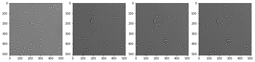
Videos#
If an image dataset has a temporal dimension, we call it a video. Processing videos works similar to multi-channel images and image stacks. Let’s open a microscopy dataset showing yeast cells rounding over time. (Image data courtesy of Anne Esslinger, Alberti lab, MPI CBG)
video = imread('../../data/rounding_assay.tif')

video.shape
(64, 512, 512)
fig, axs = plt.subplots(1, 4, figsize=(15,15))

# show three planar images
axs[0].imshow(video[0], cmap='Greys_r')
axs[1].imshow(video[5], cmap='Greys_r')
axs[2].imshow(video[10], cmap='Greys_r')
axs[3].imshow(video[15], cmap='Greys_r');
n-dimensional data#
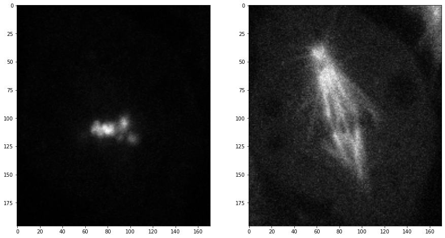
High-dimensional data are pretty common in microscopy. To process them correctly, one must study carefully what dimensions an image dataset has. We can explore possibilities using the mitosis dataset:
mitosis = imread('../../data/mitosis.tif')

mitosis.shape
(51, 5, 2, 196, 171)
Hint: Open the dataset in ImageJ/Fiji to understand what these numbers stand for. You can see there that the mitosis dataset has
51 frames,
5 Z-slices,
2 channels and
is 171 x 196 pixels large.
We grab now channels 1 and 2 of the first time point (index 0) in the center plane (index 2):
timepoint = 0
plane = 2

channel1 = mitosis[timepoint, plane, 0]
channel2 = mitosis[timepoint, plane, 1]

fig, axs = plt.subplots(1, 2, figsize=(15,15))

axs[0].imshow(channel1, cmap='Greys_r')
axs[1].imshow(channel2, cmap='Greys_r');
Exercise#
Open the mitosis dataset, select three timepoints and show them side-by-side. The resulting figure should have three columns and two rows. In the first row, channel1 is displayed and the second channel below.