Filter overview#
In this notebook we demonstrate some more typical filters using the nuclei example image.
import numpy as np

import matplotlib.pyplot as plt
from skimage.io import imread
from skimage import data
from skimage import filters
from skimage import morphology
from scipy.ndimage import convolve, gaussian_laplace
import stackview
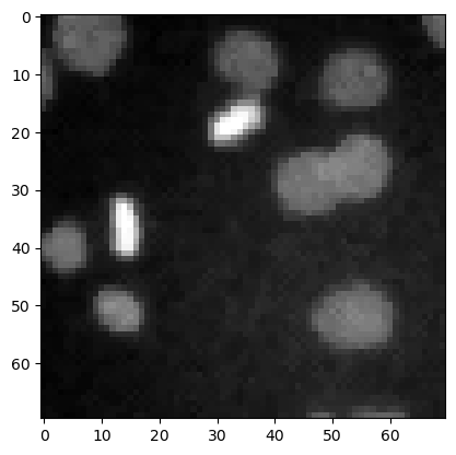
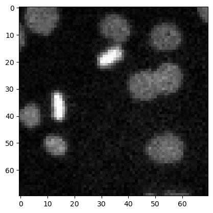
image3 = imread('../../data/mitosis_mod.tif').astype(float)

plt.imshow(image3, cmap='gray')
<matplotlib.image.AxesImage at 0x12d1b7ce940>

Denoising#
Common filters for denoising images are the mean filter, the median filter and the Gaussian filter.
denoised_mean = filters.rank.mean(image3.astype(np.uint8), morphology.disk(1))

plt.imshow(denoised_mean, cmap='gray')
<matplotlib.image.AxesImage at 0x12d1ba2df10>

denoised_median = filters.median(image3, morphology.disk(1))

plt.imshow(denoised_median, cmap='gray')
<matplotlib.image.AxesImage at 0x12d1b8ef340>
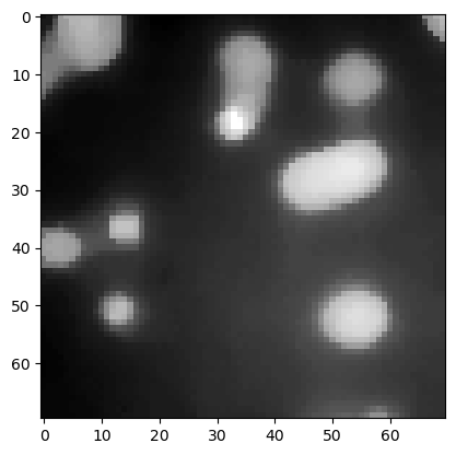
denoised_median2 = filters.median(image3, morphology.disk(5))

plt.imshow(denoised_median2, cmap='gray')
<matplotlib.image.AxesImage at 0x12d1b96bb20>
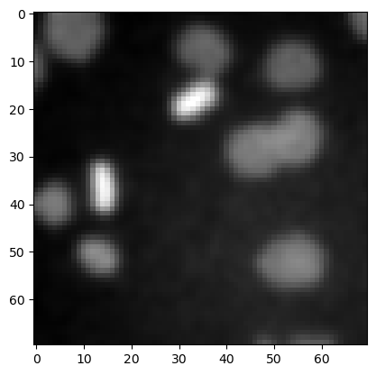
denoised_gaussian = filters.gaussian(image3, sigma=1)

plt.imshow(denoised_gaussian, cmap='gray')
<matplotlib.image.AxesImage at 0x12d1bbbb880>
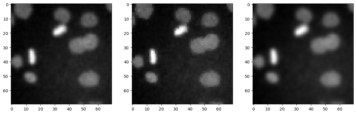
We can also show these images side-by-side using matplotlib.
fig, axes = plt.subplots(1,3, figsize=(15,15))

axes[0].imshow(denoised_mean, cmap='gray')
axes[1].imshow(denoised_median, cmap='gray')
axes[2].imshow(denoised_gaussian, cmap='gray')
<matplotlib.image.AxesImage at 0x12d1bae6d60>
Top-hat filtering / background removal#
top_hat = morphology.white_tophat(image3, morphology.disk(15))

plt.imshow(top_hat, cmap='gray')
<matplotlib.image.AxesImage at 0x12d1d549c10>
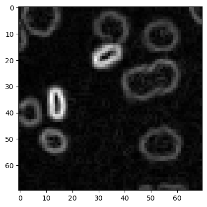
Edge detection#
sobel = filters.sobel(image3)

plt.imshow(sobel, cmap='gray')
<matplotlib.image.AxesImage at 0x12d1ccc6bb0>
Exercise#
Apply different radii for the top-hat filter and show them side-by-side.