Explaining Object classification using SHAP

In this notebook, we will segment objects in an image and classify them using shape measurements. Using SHAP Analysis we can explain what role the different shape descriptors play.

import numpy as np
from skimage.io import imread
from skimage.measure import label, regionprops_table
import pandas as pd
from sklearn.ensemble import RandomForestClassifier
from sklearn.model_selection import train_test_split
import shap
import stackview

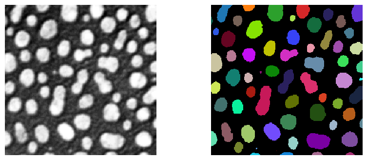
We use the blobs example image which contains multiple objects which could be grouped according to their size and shape. For example the 8-shaped objects in the center could be identified as group.

# Load the image
image = imread('data/blobs.tif')
# Apply threshold and 
binary = image > 120
# Label connected components
labels = label(binary)

import stackview
from matplotlib import pyplot as plt

fig, ax = plt.subplots(1, 2, figsize=(10, 4))
stackview.imshow(image, plot=ax[0])
stackview.imshow(labels, plot=ax[1]) 

Extract region properties

To allow object classification using shape features, we need to measure and compute the features.

# Measure object properties using scikit-image
properties = ['label', 'area', 'perimeter', 'mean_intensity', 'max_intensity', 
             'min_intensity', 'eccentricity', 'solidity', 'extent', "minor_axis_length", "major_axis_length"]
measurements = regionprops_table(labels, intensity_image=image, properties=properties)
df = pd.DataFrame(measurements)
# Add aspect ratio column
df['aspect_ratio'] = df['major_axis_length'] / df['minor_axis_length']

display(df.head())

	label	area	perimeter	mean_intensity	max_intensity	min_intensity	eccentricity	solidity	extent	minor_axis_length	major_axis_length	aspect_ratio
0	1	433.0	91.254834	190.854503	232.0	128.0	0.876649	0.881874	0.555128	16.819060	34.957399	2.078439
1	2	185.0	53.556349	179.286486	224.0	128.0	0.828189	0.968586	0.800866	11.803854	21.061417	1.784283
2	3	658.0	95.698485	205.617021	248.0	128.0	0.352060	0.977712	0.870370	28.278264	30.212552	1.068402
3	4	434.0	76.870058	217.327189	248.0	128.0	0.341084	0.973094	0.820416	23.064079	24.535398	1.063793
4	5	477.0	83.798990	212.142558	248.0	128.0	0.771328	0.977459	0.865699	19.833058	31.162612	1.571246

Annotation data

Next we load some annotation data. The annotation was hand-drawn on a label image and needs to be converted to tabular format first.

# Load annotation image and extract maximum intensity per label
annotation_image = imread('data/blobs_label_annotation.tif')
annotation_props = regionprops_table(labels, intensity_image=annotation_image, 
                                    properties=['label', 'max_intensity'])
annotation_df = pd.DataFrame(annotation_props)
annotation_df = annotation_df.rename(columns={'max_intensity': 'annotation'})

# Merge with main dataframe
df = df.merge(annotation_df, on='label')
display(df.head())

	label	area	perimeter	mean_intensity	max_intensity	min_intensity	eccentricity	solidity	extent	minor_axis_length	major_axis_length	aspect_ratio	annotation
0	1	433.0	91.254834	190.854503	232.0	128.0	0.876649	0.881874	0.555128	16.819060	34.957399	2.078439	0.0
1	2	185.0	53.556349	179.286486	224.0	128.0	0.828189	0.968586	0.800866	11.803854	21.061417	1.784283	0.0
2	3	658.0	95.698485	205.617021	248.0	128.0	0.352060	0.977712	0.870370	28.278264	30.212552	1.068402	2.0
3	4	434.0	76.870058	217.327189	248.0	128.0	0.341084	0.973094	0.820416	23.064079	24.535398	1.063793	0.0
4	5	477.0	83.798990	212.142558	248.0	128.0	0.771328	0.977459	0.865699	19.833058	31.162612	1.571246	0.0

len(df)

64

Train Random Forest Classifier

Next, we train a random forest classifier. Therefore, we exctract only the objects which were annotated.

annotated_df = df[df['annotation'] != 0]
len(annotated_df)

12

# Prepare data for classification
feature_columns = ["solidity", "perimeter", "area", "aspect_ratio", "extent"]
                  # annotated_df.columns #['area', 'perimeter', 'mean_intensity', 'max_intensity', 
                  # 'min_intensity', 'eccentricity', 'solidity', 'extent']
X = annotated_df[feature_columns]
y = annotated_df['annotation']

# Split data
X_train, X_test, y_train, y_test = train_test_split(X, y, test_size=0.2, random_state=42)

# Train model
rf = RandomForestClassifier(n_estimators=100, random_state=42)
rf.fit(X_train, y_train)

# Print accuracy
print(f"Training accuracy: {rf.score(X_train, y_train):.3f}")
print(f"Testing accuracy: {rf.score(X_test, y_test):.3f}")

Training accuracy: 1.000
Testing accuracy: 0.333

We can now apply this classifier to the entire dataset.

y_ = rf.predict(df[feature_columns])
y_

array([1., 3., 3., 3., 3., 3., 2., 3., 3., 1., 3., 3., 2., 3., 3., 1., 3.,
       3., 3., 3., 3., 3., 1., 3., 3., 3., 1., 3., 3., 3., 1., 2., 1., 3.,
       3., 1., 3., 1., 3., 3., 2., 3., 3., 3., 3., 3., 3., 3., 1., 3., 3.,
       1., 3., 3., 3., 1., 3., 3., 3., 2., 1., 3., 1., 1.])

# Map labels to y values
result = labels.copy()
for i, label_id in enumerate(np.unique(labels)[1:], 1):  # skip 0 as it's background
    result[labels == label_id] = y_[i-1]

# Show result
stackview.insight(result)

shape (254, 256) dtype int32 size 254.0 kB min 0 max 3 n labels 3

Explain classification using SHAP values

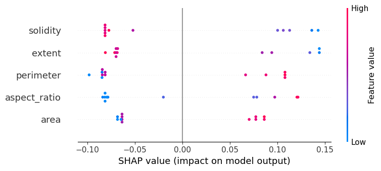
Using the SHAP-plot we can determine which features contribute most to the decision of the classifier. The plot below can be interpreted like this:

• The solidity and extend features contribute most to the classification. If solidity abd extend are low (blue), the object might be 8-shaped.

• Also perimeter and aspect_ratio contribute. If they are high, the object might be 8-shaped.

• The area contributes as well, just a little les prominently. If objects are large, they are more likely to be 8-shaped.

explainer = shap.TreeExplainer(rf)
shap_values = explainer.shap_values(X)[...,0]

shap.summary_plot(shap_values, X) #, feature_names=feature_columns)

Exercise

Draw the SHAP summary plot for the shap values [..., 1]. Which object class was this SHAP plot drawn for?