Micro-sam for instance segmentation

In this notebook, we want to try out automatic instance segmentation using micro-sam.

It is inspired by the automatic-segmentation notebook in the micro-sam github repository as well as two introductory notebooks written by Robert here and here.

You can install micro-sam in a conda environment like this. If you never worked with conda-environments before, consider reading this blog post first.

conda install -c conda-forge micro_sam

Let us first import everything we need:

from micro_sam.automatic_segmentation import get_predictor_and_segmenter, automatic_instance_segmentation
from skimage.io import imread
import matplotlib.pyplot as plt

INFO:OpenGL.acceleratesupport:No OpenGL_accelerate module loaded: No module named 'OpenGL_accelerate'

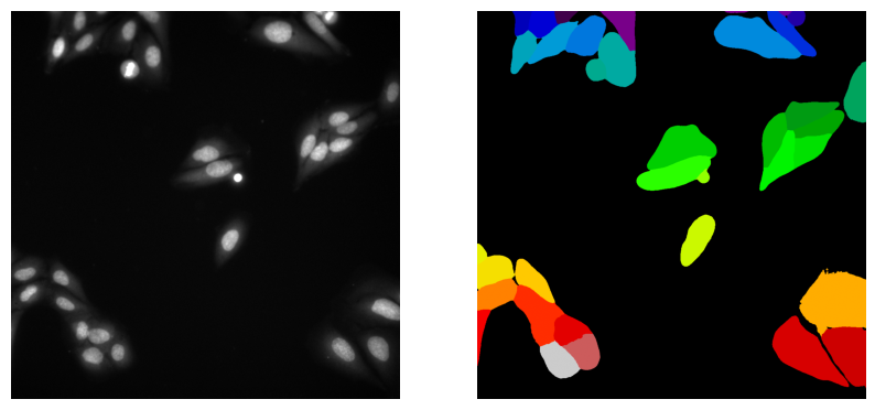
As an example image, we use a fluorescence microscopy dataset published by M. Arvidsson et al. showing Hoechst 33342-stained nuclei, licensed CC-BY 4.0.

# Load microscopy image
image = imread("../../data/development_nuclei.png")

# Show input image
plt.imshow(image, cmap="gray")

<matplotlib.image.AxesImage at 0x3101db830>

First, we load a segmentation model and its helper (predictor and segmenter) that are trained to recognize and separate different structures in an image. Then, we apply them to our input image to create a label image (label_image), where each detected object is assigned a unique label, making the segmentation ready for further analysis.

# Load model
predictor, segmenter = get_predictor_and_segmenter(model_type="vit_b_lm")

# Apply model
label_image = automatic_instance_segmentation(predictor=predictor, segmenter=segmenter, input_path=image)

Using apple MPS device.

Compute Image Embeddings 2D: 100%|██████████| 1/1 [00:01<00:00,  1.03s/it]
Initialize instance segmentation with decoder: 100%|██████████| 1/1 [00:00<00:00,  2.90it/s]

Now, we can investigate the results.

# show image and label image side-by-sid
plt.figure(figsize=(10, 5))
plt.subplot(1, 2, 1)
plt.imshow(image, cmap="gray")
plt.axis("off")
plt.subplot(1, 2, 2)
plt.imshow(label_image, cmap="nipy_spectral")
plt.axis("off")
plt.show()

If you want to dive further into this topic, see the linked jupyter notebooks as well as this video playlist.

Exercise

We have used the model vit_b_lm. Try out another one, for example vit_b_em_organelles which is specialized for electron microscopy and organelle segmentation. Which differences in the segmentation result can you observe and why do you think this is the case?